当前位置：文档库 › Design of a rail transit line for profit maximization in a linear transportation corridor

Design of a rail transit line for profit maximization in a linear transportation corridor

Design of a rail transit line for pro?t maximization in a linear transportation corridor

Zhi-Chun Li a ,b ,William https://www.wendangku.net/doc/615622352.html,m a ,?,S.C.Wong c ,A.Sumalee a

Department of Civil and Structural Engineering,The Hong Kong Polytechnic University,Kowloon,Hong Kong,China b

School of Management,Huazhong University of Science and Technology,Wuhan 430074,China c

Department of Civil Engineering,The University of Hong Kong,Pokfulam Road,Hong Kong,China

a r t i c l e i n f o Keywords:

Transportation corridor Rail line design

Pro?t maximization Population density

Transit pricing structure Urban form

a b s t r a c t

This paper addresses the design problem of a rail transit line located in a linear urban transportation corridor.The service variables designed are a combination of rail line length,number and locations of stations,headway and fare.Two pro?t maximization models,which account for the effects of different transit pricing structures (?at and distance-based fare regimes),are proposed.In the proposed models,the effects of passenger demand elas-ticity and population density along the urban corridor are explicitly considered.The solu-tion properties of the proposed models are explored and compared analytically,and the indifference condition for the two fare regimes in terms of the operator’s net pro?t is iden-ti?ed.A heuristic solution algorithm to solve the proposed models is presented.Numerical examples are provided to show the effects of the fare regimes,rail capital cost and urban con?guration (in terms of urban population distribution and corridor length)on the design of the rail transit line and the pro?tability of the rail transit operations.

1.Introduction

1.1.Background and motivation

Over the past few decades,rapid urban expansion due to urbanization and economic growth in some large Asian cities,including Shanghai and Hong Kong,has drastically increased the size of these cities.Traf?c congestion has worsened due to the shortage of space for road expansion projects to accommodate the growing traf?c demand in urban areas.To address this problem,the local authorities of these cities have launched rail transit development projects,which include extension of existing rail transit lines and construction of new rail transit lines.For instance,the Shanghai municipal government is cur-rently extending Rail Line 11about 5.76km westwards and creating four new stations on the line,while the Hong Kong gov-ernment recently approved a proposal to build a new metro line to connect Shatin New Town to Central (i.e.,the central business district (CBD)of Hong Kong),with a total length of 17km and 10stations.The construction of this new metro pro-ject is expected to start in 2011and be completed in 2019.

In principle,the basic parameters to be determined in planning a rail transit line project include the rail line length,num-ber and locations of stations,headway and fare (see,e.g.Vuchic,2005;and the references shown in Table 1).The design of these parameters depends very much on the population density in the planning area.This is because the urban population

?Corresponding author.Tel.:+852********;fax:+852********.

E-mail addresses:smzcli@https://www.wendangku.net/doc/615622352.html, (Z.-C.Li),cehklam@https://www.wendangku.net/doc/615622352.html,.hk (https://www.wendangku.net/doc/615622352.html,m),hhecwsc@hkucc.hku.hk (S.C.Wong),ceasumal@https://www.wendangku.net/doc/615622352.html,.hk (A.Sumalee).

density directly in?uences the level of passenger demand.For instance,in a sparsely populated city (e.g.many Western cit-ies),operators prefer to short rail transit lines in order to minimize their costs (Spasovic and Schonfeld,1993;Spasovic et al.,1994).However,in a densely populated city,such as Hong Kong in which most people use transit services for their daily travel,a bene?t-driven operator has an incentive to extend the rail transit line from the city’s CBD area into its outer areas so as to procure more pro?t.It is,therefore,important to address the relationship between the design parameters of the rail transit line and the urban population density.

Obviously,there are various tradeoffs between the extension of a rail transit line and its associated costs.For instance,the length of a rail line is closely related to its service coverage and its capital and operating costs.A longer rail line pro-vides greater service coverage but incurs higher capital and operating costs,whereas a shorter rail line has lower capital and operating costs but offers less service coverage.The station spacing along a rail line directly affects the train operating speed and train dwell time at stations,and thus passenger demand on that line.In general,shorter station spacing can decrease the average passenger access time to stations.However,it also increases the average passenger in-vehicle travel time and train operating costs because of higher acceleration and deceleration delays caused by frequent stops.Con-versely,longer station spacing can increase the train operating speed and decrease the average passenger in-vehicle travel time,but also increases the average passenger access time to stations.Since these tradeoffs are directly related to the rev-enues and thus pro?ts of the rail transit operations,all of these parameters –the rail line length,number and spacing of stations,headway and fare –should be carefully designed.The present study addresses this design problem for strategic planning purposes.1.2.Literature review

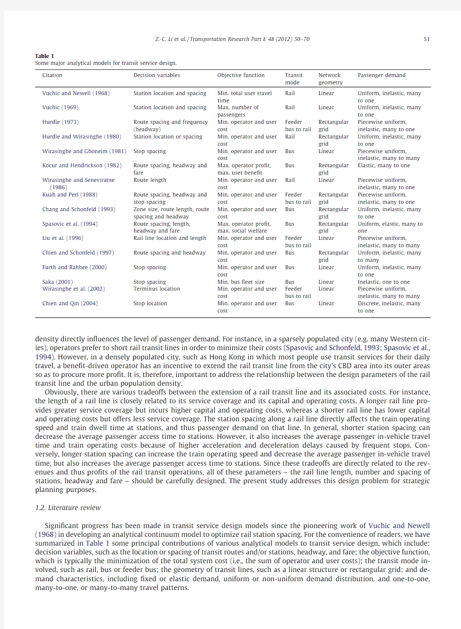
Signi?cant progress has been made in transit service design models since the pioneering work of Vuchic and Newell (1968)in developing an analytical continuum model to optimize rail station spacing.For the convenience of readers,we have summarized in Table 1some principal contributions of various analytical models to transit service design,which include:decision variables,such as the location or spacing of transit routes and/or stations,headway,and fare;the objective function,which is typically the minimization of the total system cost (i.e.,the sum of operator and user costs);the transit mode in-volved,such as rail,bus or feeder bus;the geometry of transit lines,such as a linear structure or rectangular grid;and de-mand characteristics,including ?xed or elastic demand,uniform or non-uniform demand distribution,and one-to-one,many-to-one,or many-to-many travel patterns.

Table 1

Some major analytical models for transit service design.Citation

Decision variables

Objective function Transit mode Network geometry Passenger demand Vuchic and Newell (1968)Station location and spacing Min.total user travel time

Rail Linear Uniform,inelastic,many to one

Vuchic (1969)Station location and spacing Max.number of passengers

Rail Linear Uniform,inelastic,many to one

Hurdle (1973)

Route spacing and frequency (headway)

Min.operator and user cost

Feeder bus to rail Rectangular grid

Piecewise uniform,inelastic,many to one Hurdle and Wirasinghe (1980)Station location or spacing Min.operator and user cost

Rail Rectangular grid Uniform,inelastic,many to one

Wirasinghe and Ghoneim (1981)Stop spacing

Min.operator and user cost

Bus Linear Piecewise uniform,

inelastic,many to many Kocur and Hendrickson (1982)Route spacing,headway and fare

Max.operator pro?t,https://www.wendangku.net/doc/615622352.html,er bene?t

Bus Rectangular grid Elastic,many to one Wirasinghe and Seneviratne (1986)

Route length

Min.operator and user cost

Rail Linear Piecewise uniform,inelastic,many to one Kuah and Perl (1988)Route spacing,headway and stop spacing

Min.operator and user cost

Feeder bus to rail Rectangular grid

Piecewise uniform,inelastic,many to one Chang and Schonfeld (1993)Zone size,route length,route spacing and headway Min.operator and user cost

Bus Rectangular grid

Uniform,inelastic,many to one

Spasovic et al.(1994)Route spacing,length,headway and fare

Max.operator pro?t,max.social welfare Bus Rectangular grid Uniform,elastic,many to one

Liu et al.(1996)

Rail line location and length Min.operator and user cost

Feeder bus to rail Linear Piecewise uniform,

inelastic,many to many Chien and Schonfeld (1997)Route spacing and headway Min.operator and user cost

Bus Rectangular grid Uniform,inelastic,many to many

Furth and Rahbee (2000)Stop spacing Min.operator and user cost

Bus Linear Uniform,inelastic,many to one

Saka (2001)

Stop spacing

Min.bus ?eet size

Bus Linear Inelastic,one to one Wirasinghe et al.(2002)Terminus location Min.operator and user cost

Feeder bus to rail Linear Piecewise uniform,

inelastic,many to many Chien and Qin (2004)

Stop location

Min.operator and user cost

Bus

Linear

Discrete,inelastic,many to one

Z.-C.Li et al./Transportation Research Part E 48(2012)50–70

52Z.-C.Li et al./Transportation Research Part E48(2012)50–70

Most existing transit models,as shown in Table1,usually aim to minimize the sum of operator and user costs.This can be attributed to the relatively low population densities within large Western cities leading to government subsidy to the transit industry.However,this is not the case in some Eastern Asian cities,particularly those with high-density population devel-opment,such as Hong Kong,in which the transit industry can operate pro?tably without government subsidy.This is be-cause a large proportion of the population in Hong Kong uses transit services as the main mode of transportation,and over90%of the11million daily person-trips are served by privately operated public transit modes(Transport Department, 2003).Under Hong Kong’s operating environment,the principal objective of private transit operators is neither welfare gain nor the ef?cient utilization of road space,but rather pro?t maximization(Lam and Zhou,2000;Zhou et al.,2005;Li et al., 2009).It is thus important to address the interrelation between the population density and the transit operator’s pro?t.

The literature review also reveals that the focuses of the previous related studies have mainly been on how to optimize the design variables of the transit services approximately and/or numerically.Little attention has been paid,however,to investigating the solution properties of transit design problems,such as the concavity of objective functions concerned with regard to their decision variables.In addition,there is scant research into the effects of different transit pricing structures.In reality,a?at fare regime and a distance-based one can have signi?cantly different effects on the attractiveness of transit ser-vices and the level of passenger demand.

1.3.Problem statement and contributions

To address the foregoing issues,this paper develops analytical models for designing the service variables of a rail transit line located in a linear transportation corridor of length B,as shown in Fig.1.In this?gure,the rail line designed extends from the CBD of the city outward,and is represented by an ordered sequence of stations{1,2,...,N+1}.The symbol D s rep-resents the distance of station s from the CBD,and D1the length of the rail line.The service variables designed include the rail line length,D1;number of stations,N+1;station locations,D s,s=2,...,N;train headway,H;and fare for traveling from sta-tion s to the CBD,f s.For presentation purpose,all variables and parameters used throughout this paper are de?ned in Table2.

This paper makes three main contributions to the previous related studies.First,in order to examine the effects of differ-ent transit pricing regimes(?at and distance-based fare regimes),two pro?t maximization models are proposed.Second,the solution properties of the proposed models,particularly those with uniform population density and/or even(average)station spacing,are explored and compared analytically.The indifference condition of the operator’s net pro?ts for the?at and dis-tance-based fare regimes is also identi?ed.Third,a heuristic solution algorithm to solve the proposed models is developed. With the proposed models and solution algorithm,effects of some key model parameters,such as population density,rail capital cost and corridor length,are examined and evaluated in this paper.

The remainder of this paper is organized as follows.In the next section,some basic model assumptions are described and the passenger demand for each station is de?ned.Section3presents the pro?t maximization models for the?at and dis-tance-based fare regimes,respectively.The solution properties of the two proposed models are then examined and dis-cussed.In addition,the constraint conditions of the models are also presented.In Section4,a heuristic solution algorithm is developed for jointly solving the design variables of the rail transit line.In Section5,an example is used to illustrate the application of the proposed models and solution algorithm.Finally,conclusions are given in Section6together with rec-ommendations for further studies.

2.Basic considerations

2.1.Assumptions

To facilitate the presentation of the essential ideas without loss of generality,the following basic assumptions are made in this paper.

A1The corridor connecting the city’s CBD and suburb is assumed to be linear,following the previous related studies

including those of Wang et al.(2004)and Liu et al.(2009)and some listed in Table 1.

A2The study period is assumed to be a one-hour period,such as the morning peak hour,which is usually the most critical

period in a day.Therefore,this paper mainly focuses on a many-to-one travel demand pattern.

A3Passengers are assumed to board trains at the nearest rail station in terms of access time.Trains running along the rail

line stop at each station on that line,and the average train dwell time at each station is assumed to be a constant.These assumptions have also been adopted in some previous related studies,such as those of Wirasinghe and Gho-neim (1981),Kuah and Perl (1988),Chien and Schonfeld (1997),Chien and Schonfeld (1998),and Chien and Qin (2004),but can be relaxed in further studies.

A4The population density along the corridor is speci?ed as a negative exponential function (see,e.g.Anas,1982;O’Sul-livan,2000).We represent the population density at distance x from the CBD as g (x )=g 0exp(àh x ),"x 2[0,B ],where g 0is the population density in the CBD and h (P 0)is the density gradient describing how rapidly the density falls as the distance increases (see Fig.5later).The larger the value of h ,the smaller the population density at the city’s edge and the more compact the city.That is,a smaller value of h means a more decentralized city.In particular,when h equals 0,the negative exponential population density function is reduced to a uniform one.With this assumption,the total

number of population G in the study area is then given by G ?R B

0g 0exp eàh x Tdx .

Table 2Notation.Symbol De?nition

Baseline value B Length of transportation corridor (km)–C Total cost ($/h)

–C O Train operating cost ($/h)–C L Rail line cost ($/h)–C S Rail station cost ($/h)

–D s Distance of station s from the CBD;D =(D s ,s =1,2,...,N )is the corresponding vector (km)–e a Sensitivity parameter for access time (1/h)0.98e w Sensitivity parameter for wait time (1/h)

0.98e t Sensitivity parameter for in-vehicle time (1/h)0.49e f Sensitivity parameter for fare (1/$)

0.098f s Fare for traveling from station s to the CBD ($for ?at fare,$/km for distance-based fare)–F Fleet size (or number of trains)on the rail line (vehicles)–g (x )Population density at distance x from the CBD (persons/km 2)–g 0Population density in the CBD (persons/km 2)

–G Total number of population in the planning area (persons)–H Train headway (h/vehicle)

–K Capacity of vehicles,including seated and standing passengers (pass/veh)1800L s

Distance of the passenger watershed line l s from the CBD (km)–N +1Total number of stations on the rail line

–P (x )Potential passenger demand density at location x (pass/km h)

–P 0

Potential passenger demand density in the CBD;P 0=/g g 0(pass/km h)–q (x ,s )Density of passenger demand for station s at location x (pass/km h)–Q s Passenger demand for station s (pass/h)–R Total revenue of rail transit operator ($/h)

–t s Average passenger in-vehicle time from station s to the CBD (h)–T s 1Non-stop line-haul travel time from station s to the CBD (h)–T s 2Total train dwell time from station s to the CBD (h)–T 0Constant terminal time on the circular line (h)

0.08u s (x )Passenger access time to station s from location x (h)–V t Average train cruise speed (km/h)

40V a Average walking speed of passengers (km/h) 4.0w s

Average passenger wait time at station s (h)

–p Net pro?t of operator ( p

for ?at fare regime,and ^p for distance-based fare regime)($/h)–a

Ratio of passenger waiting time to train headway 0.5b 0

Average train dwell time at a rail station (h)0.01c 0Fixed component of rail line cost ($/h)

750c 1Variable component of rail line cost ($/km h)300l 0Fixed component of train operating cost ($/h)

1350l 1

Variable component of train operating cost ($/veh h)540K 0Fixed component of rail station cost ($/h)

1250K 1Variable component of rail station cost ($/station h)500H Vehicle round journey time on the rail line (h)

–h

Density gradient describing how rapidly the density falls as the distance increases (1/km)–g

Average number of trips to the CBD per person per day

1.0/Peak-hour factor,i.e.the ratio of peak-hour ?ow to daily average ?ow 0.1f

Number of terminal times on the rail line

1.0

Z.-C.Li et al./Transportation Research Part E 48(2012)50–70

A5An elastic demand density function is de?ned to capture the responses of passengers to the quality of the rail transit line service,which is measured by a generalized travel cost that is a weighted combination of the access time to sta-tions,wait time at stations,in-vehicle time,and fare.The responses include the decision of switching to an alternative mode(e.g.,auto,bus,or walk)and the decision of not making the journey at all(Li et al.,2009).

2.2.Passenger demand for each station

As both stations on any segment of the rail line are competing for passengers between those two stations,there exists a passenger watershed line that divides the line segment between two adjacent stations into two sub-segments,as shown in Fig.1.The passengers in the two sub-segments respectively use the upstream and downstream stations of the line segment. Let l s be the passenger watershed line between stations s and s+1,and L s be the distance of the passenger watershed line l s from the CBD.Based on A3,the watershed line l s is located at the middle point of the line segment(s,s+1),which implies

L s?D stD st1

;8s?1;2;...;Ne1T

where D N+1=0.

Let q(x,s)denote the density of passenger demand(i.e.the number of passengers per unit of distance)for station s at loca-tion x.The total passenger demand for station s,Q s,is then given by

Q s?

Z L sà1

L s

qex;sTdx;8s?1;2;...;Ne2T

where L s,s=1,2,...,N can be given by Eq.(1).L0represents the maximum location that the residents between station1and the corridor boundary will use the rail service,as shown in Fig.1.Beyond that location(i.e.x>L0),no one will patronize the rail system.Thus,L0holds

qeL0;1T?0;L02?D1;B e3T

where q(L0,1)is the density of passenger demand for station1at location L0.

In order to determine q(x,s),we?rst de?ne the potential passenger demand density at location x,which is denoted by P(x).De?ne g as the average number of trips to the CBD per person per day within the study area,then g g(x)is the potential passenger demand density at location x per day in terms of A4.Let/be the peak-hour factor,i.e.the ratio of peak-hour?ow to the daily average?ow.P(x)can then be given by

PexT?/g g0expeàh xT?P0expeàh xT;8x2?0;B e4Twhere P0is the(peak-hour)potential passenger demand density in the CBD and P0=/g g0.The parameter/is used to convert the traf?c volume from a daily basis to an hourly basis.

Passenger demand for rail line service is usually sensitive to rail fare level and various time components(walk/access time to station,wait time and in-vehicle time)and thus is elastic.In order to model the effects of passenger demand elas-ticity,in this paper a linear elastic demand density function is used and speci?ed as

qex;sT?PexTe1àe a u sexTàe w w sàe t t sàe f f sT;8x2?0;B ;s?1;2;...;Ne5T

where u s(x)is the passenger access time to station s from location x,which is related to the distance of location x from station s;w s is the average passenger wait time at station s;t s is the passenger in-vehicle time from station s to the CBD;and f s is the fare for traveling from station s to the CBD.e a,e w,e t and e f are the sensitivity parameters for the access time,wait time,in-vehicle time and fare,respectively.

To ensure the non-negativity of the passenger demand,the following condition should be satis?ed 061àe a u sexTàe w w sàe t t sàe f f s61;8x2?L s;L sà1 ;s?1;2;...;Ne6TIt should be pointed out that the parameters e a,e w,e t and e f in the linear demand function(5)are not the actual measures of demand elasticities.The ratios e a/e f,e w/e f and e t/e f determine the values of access time,wait time and in-vehicle time,respec-tively.The value of walking/access time is generally larger than the value of in-vehicle time(Chang and Schonfeld,1991),and thus e a>e t holds.

In addition,the linear demand function,as adopted here,has been extensively used in demand models due to its conve-nience for analytical tractability.Other alternative demand functions,such as exponential demand function,can also be adopted.However,it is usually dif?cult,if not impossible,to derive a closed-form solution.Alternatively,a non-linear de-mand function can be approximated as a linear demand function by using the?rst-order Taylor series expansion.

We now de?ne the time components that are included in the linear demand function(5).The passenger access time u s(x) depends on the walking distance between location x and station s and the walking speed of passengers,V a.It is expressed as

u sexT?

eD sàxT=V a;8x6D s

exàD sT=V a;8x>D s

;8x2?0;B ;s?1;2;...;Ne7T

54Z.-C.Li et al./Transportation Research Part E48(2012)50–70

The average passenger wait time at station s,w s,can be calculated by

w s?a H;8s?1;2;...;Ne8Twhere H is the headway of the rail service,and a is a calibration parameter that depends on the distributions of train head-way and passenger arrival.The value a=0.5is commonly used to suggest a constant headway between trains and a uniform random passenger arrival distribution.

The passenger in-vehicle time from station s to the CBD,t s,comprises the non-stop line-haul travel time,T s1,and train dwell time,T s2,at rail stations,i.e.,

t s?T s1tT s2;8s?1;2;...;Ne9Twhere T s1can be calculated by the in-vehicle length of the trip being made by the passengers divided by the average train cruise speed,V t,i.e.,

T s1?D s

V t

;8s?1;2;...;Ne10T

According to A3,the average train dwell time at each rail station is a constant.Consequently,the total train dwell time from station s to the CBD,T s2,can be calculated by

T s2?b0eNt1àsT;8s?1;2;...;Ne11Twhere b0is the average train dwell time at a station,which can be calibrated with observed data(Lam et al.,1998).

Substituting Eqs.(5)–(11)into Eq.(2),Q s can then be rewritten as

Q s?k s

Z L sà1

L s PexTdxà

e a

Z D s

L s

PexTeD sàxTdxt

Z L sà1

D s

PexTexàD sTdx

;8s?1;2;...;Ne12T

where

k s?1àe w w sàe t t sàe f f s?1àe w a Hàe t

D s

V t

tb0eNt1àsT

àe f f s;8s?1;2;...;Ne13T

On the basis of Eqs.(3)–(13),the maximum service coverage L0of the rail transit line can be given by

L0?D1tV a

e a

k1e14T

where k1can be determined by Eq.(13).

3.Model formulation

3.1.Pro?t maximization models

As previously stated,the objective of the rail transit operator is to maximize its net pro?t.The net pro?t,denoted as p,is the total revenue,R,which is generated from the passenger fares,minus the total cost,C.It is expressed as p?RàCe15TIn the following,we?rst de?ne the total cost C.As described in Chien and Schonfeld(1997,1998),the total cost C is incurred by train operations,rail line,and rail stations,and thus consists of the following three cost components:train operating cost, C O;rail line cost,C L;and rail station cost,C S.It is represented as

C?C OtC LtC Se16TThe train operating cost C O comprises the?xed operating cost,l0,and variable operating cost,l1F,where F is the?eet size (or the number of trains)on that line and l1is the hourly operating cost per train.It is formulated as

C O?l0tl1Fe17Twhere F equals the vehicle round journey time,H,divided by headway H,i.e.,

F?H

e18T

where the round journey time H comprises the terminal time,line-haul travel time and train dwell time at stations,which is expressed as

H?f T0t2eT11tT12Te19Twhere T0is the constant terminal time on the circular line and f is the number of terminal times on the line.T11and T12are, respectively,the total line-haul travel time and total dwell time for train operations from station1to the CBD.From Eqs.(10) and(11),we have T11=D1/V t and T12=b0N.

Z.-C.Li et al./Transportation Research Part E48(2012)50–7055

The rail line cost,C L ,is the sum of the ?xed costs,c 0(e.g.,line overhead cost),and variable costs,c 1D 1(e.g.,land acqui-sition,line construction,maintenance,and labor costs),proportional to the rail line length D 1;i.e.,

C L ?c 0tc 1

D 1

e20T

where c 1is the hourly rail line operating cost per kilometer.

The rail station cost,C S ,includes ?xed costs (e.g.,station overhead cost)and variable costs (e.g.,station land acquisition,design and construction,operating,and maintenance costs).The total variable cost is determined by the number of stations multiplied by the average unit station cost.C S can thus be expressed as

C S ?K 0tK 1eN t1Te21T

where K 0is the ?xed cost for station operations and K 1is the hourly operating cost per station.

We now de?ne the total operating revenue R that appears in Eq.(15).It is the sum of the number of passengers boarding at each station multiplied by the corresponding fare,i.e.,

R ?

X N s ?1

f s Q s e22T

where the passenger demand for station s ,Q s ,is given by Eq.(12).The transit fare f s depends on the fare regimes adopted.

Different transit fare regimes can lead to different levels of operating revenue and thus pro?t of the operator.In this pa-per,we consider two types of fare regimes:a ?at fare regime in which all passengers are charged the same fare regardless of the length of their trips,and a distance-based regime in which the fares grow linearly with the distance travelled by passen-gers.Mathematically,the two fare regimes are,respectively,represented as follows.For the ?at fare regime,

f s ? f ;

8s ?1;2;...;N e23T

where f is a constant.

For the distance-based fare regime,

f s ?f 0t^f D s ;

8s ?1;2;...;N e24T

where f 0and ^f are the ?xed and variable components of the distance-based fare,respectively.

In view of Eqs.(15)–(24),the pro?t maximization problems for the ?at and distance-based fare regimes can,respectively,be formulated as

max p eD ;H ; f T? f

X N s ?1

Q s à

l 0t

l 1

f T 0t2D 1

V t

t2b 0N

àec 0tc 1D 1Tà?K 0tK 1eN t1T

e25T

and

max ^p eD ;H ;^f T?

X N s ?1

ef 0t^f D s TQ s àl 0tl 1f T 0t

2D 1

t t2b 0N !àec 0tc 1D 1Tà?K 0tK 1eN t1T e26T

where the bolded symbol ‘‘D ’’is the vector of station locations,i.e.D =(D s ,"s =1,2,...,N ).Q s can be determined by Eq.(12).

The decision variables include the rail line length D 1,station locations D 2,...,D N ,train headway H ,and fare f for the ?at fare

regime or ^f for the distance-based fare regime.

The optimal solutions for the rail line length,station location (or spacing),headway and fare can be obtained by setting the partial derivatives of each objective function with respect to its decision variables equal to zero and solving them simul-taneously.We then have the following proposition (the proof is given in Appendix A ).

Proposition 1.The optimal rail line length,station location (or spacing),headway and fare solutions for the ?at and distance-based fare regimes satisfy the systems of equations as shown in Table 3,respectively.

We now look at a special case with an even station spacing,which can be regarded as the average station spacing.The even (or average)station spacing solution can serve as a benchmark indicator for the planning and design of rail transit line service,particularly at the early stage of the design of the transit line.Let d represent the even (or average)station spacing of the rail line,one then obtains D s =(N +1às )d and thus L s ?N às t1

2àád in terms of Eq.(1).Substituting them into Eqs.(12),(13),(14),(25)and (26),we can then derive the ?rst-order optimality conditions of the optimization models (25)and (26)as follows (this proof is similar to Proposition 1and omitted here).

Proposition 2.The optimal even (average)station spacing,headway and fare solutions for the ?at and distance-based fare regimes satisfy the systems of equations as shown in Table 4,respectively.

56Z.-C.Li et al./Transportation Research Part E 48(2012)50–70

3.2.Properties of models

In this section,we examine the properties of the models (25)and (26)that are proposed in the previous section.On the

basis of the ?rst-order optimality conditions presented in Table 3,the second-order partial derivatives of p

eáTwith respect to headway H and fare f are,respectively,given by

@2 p @H 2?àa e w f P eL 0T@L 0@H à2l 1H 3f T 0t2D 1V t t2b 0N ?ea e w T2 f P eL 0TV a e a à2l 1H 3f T 0t2D 1V t t2b 0N

@2 p @ f ?àe f f P eL 0T@L 0@ f

à2e f P N s ?1R L s à1L s P ex Tdx ?e 2f f P eL 0TV a a à2e f P N s ?1R L s à1L s P ex Tdx @2 p @H @ f

?àa e w P N s ?1

R L s à1L

P ex Tdx ta e w e f f P eL 0TV a a

8>>>>>>><>>>>>>>:e27T

For the distance-based fare regime,the second-order partial derivatives of ^p eáTwith respect to H and ^f can be derived as

follows:

@2^p @H 2?ea e w T2ef 0t^f D 1TP eL 0TV a a à2l 1H 3f T 0t2D 1t t2b 0N

@2^p @^f

2?ee f D 1T2ef 0t^f D 1TP eL 0Tà2e f P N s ?1D 2s R L s à1L s P ex Tdx @2^p @H @^f

?àa e w

P N s ?1

D s R L s à1L s

P ex Tdx ta e w e f D 1ef 0t^f D 1TP eL 0TV a a

8>>>>>>><>>>>>>>:e28T

Eqs.(27)and (28)show that the signs of the second-order partial derivatives of p eáTand ^p eáTwith respect to H and f (or ^f Tare

related to the maximum service coverage L 0of the rail transit line and the city’s population density.All the second-order

Table 3

Optimal rail line length,station location,headway and fare solutions for different fare regimes.Flat fare regime Distance-based fare regime

@ p @D s ? f P s t1i ?s à1@Q i @D s àD s 2l 1HV t tc 1 ?0;s ?1;...;N

H ??????????????????????????????????????l 1f T 0t2D 1V t

t2b 0N a e w f P N s ?1R L s à1

L s P ex Tdx v u u t f ?P N s ?1Q s e f

P N s ?1

R L s à1

L s

P ex Tdx

8>>>>>>>><>>>>>>>>:@^p @D s ?^f Q s tP s t1i ?s à1ef 0t^f D i T@Q i @D s àD s 2l 1HV t tc 1 ?0;s ?1;...;N

H ??????????????????????????????????????????????????l 1f T 0t2D

1V t t2b 0N a e w P N

s ?1ef 0t^f D s TR L s à1L s P ex Tdx v u u t ^f ?P N s ?1D s Q s àf 0e f P N s ?1D s R L s à1L s P ex Tdx e f

P N s ?1

D 2s

R L s à1

L s

P ex Tdx

8>>>>>>>><

>>>>>>>>:where D s =1if s =1,and 0otherwise.@Q i /@D s can be given by

@Q s à1@D s ?12P eL s à1Tàk s à1te a V a eD s à1àL s à1T ;8s ?2;...;N @Q 1@D 1?@k 1@D 1R L 0L 1P ex Tdx tk 1P eL 0T1tV a e a @k 1@D 1 à12

P eL 1T àe a V a R D 1L 1P ex Tdx àR L 0D 1P ex Tdx te a V a 12P eL 1TeD 1àL 1Tàk 1P eL 0TV a e a 1tV a e a @k 1@D 1 @Q s @D s ?@k s @D s R L s à1L s P ex Tdx t12k s P eL s à1TàP eL s TeTàe a V a R D s L s P ex Tdx àR L s à1

D s P ex Tdx te a 2V a eP eL s TeD s àL s TàP eL s à1TeL s à1àD s TT;8s ?2;...;N @Q s t1@D s ?12

P eL s Tk s t1àe a

V a eL s àD s t1T ;8s ?1;2;...;N à18

>>>>>><>>>>>>:where @k s

@D s ?àe t =V t ;for the flat fare regime àee t =V t te f ^f T;for the distance-based fare regime

;8s ?1;2;...;N .Table 4

Optimal even (average)station spacing,headway and fare solutions for different fare regimes.Flat fare regime Distance-based fare regime

@ p @d ? f P N s ?1@Q s @d à2l 1

HV t tc 1 N ?0H ??????????????????????????????????????l 1f T 0t2N d V t

t2b 0N a e w f P N s ?1R L s à1

L s P ex Tdx v u u t f ?P N s ?1Q s e f

P s ?1

R s à1

L s

P ex Tdx

8>>>>>>>><>>>>>>>>:@^p @d ?P N s ?1^f eN t1às TQ s tef 0t^f d eN t1às TT@Q s @d à2l 1HV t tc 1 N ?0H ??????????????????????????????????????????????????????????????l 1f T 0t2N d V t t2b 0N a e w P N

s ?1ef 0t^f d eN t1às TTR L s à1L s P ex Tdx v u u t ^f ?P N s ?1eN t1às TQ s àf 0e f P N s ?1eN t1às TR L s à1L s P ex Tdx d e f

P s ?1

eN t1às T

R L s à1L s

P ex Tdx

8>>>>>>>><

>>>>>>>>:where @Q s /@d can be given by

@Q 1@d ?@k 1@d R L 0L 1P ex Tdx tk 1N tV a e a @k 1@d P eL 0TàN à12àáP eL 1T àe a V a N R D 1L 1P ex Tdx àR L 0D 1P ex Tdx te a V a d 2N à12àáP eL 1Tàk 1P eL 0TV a e a N tV a e a @k 1@d

@Q s @d ?@k s @d R L s à1L s P ex Tdx tk s N às t32àáP eL s à1TàN às t12àáP eL s Tàáàe a V a eN t1às TR D s L s P ex Tdx àR L s à1D s P ex Tdx td 2e a V a N às t12àáP eL s TàN às t32

àáP eL s à1Tàá;8s ?2;...;N 8>><>>:where @k s

@d ?àeN t1às Te t =V t ;for the flat fare regime àeN t1às Tee t =V t te f ^f T;for the distance-based fare regime

;8s ?1;2;...;N .Z.-C.Li et al./Transportation Research Part E 48(2012)50–70

partial derivatives may be negative,positive,or zero.Therefore,given all other variables,the concavity of peáT(or^peáTTwith respect to H and/or f(or H and/or^fTand thus the uniqueness of the optimal headway and/or fare solutions cannot be guar-anteed.In addition,from Eqs.(27)and(28),we have

Proposition3.Given the number N and location vector D of stations,the pro?t function peáT(or^peáT)is concave with respect to H

and f(or H and^f)if and only if@2 p

@H2<0,@2 p

@ f2

<0and@2 p

@H2

@2 p

@ f2

à@2 p

@H@ f

>0(or@2^p

@H2

<0,@2^p

@^f2

<0and@2^p

@H2

@2^p

@^f2

à@2^p

@H@^f

>0)hold

simultaneously.

However,when the population density follows a uniform distribution,i.e.g(x)=g0(or,equivalently,the potential passen-ger demand density P(x)=P0.According to Eq.(4),both can be used alternately but not causing confusion),we have the fol-lowing result.

Proposition4.For the?at fare regime,given the number N of stations,headway H and fare f,when the population density along the rail line is uniformly distributed,the pro?t function peáTis concave with regard to the rail line length D1and station locations D2,D3,...,D N.

The proof of Proposition4is provided in Appendix B.Proposition4indicates that for the?at fare regime and a uniform population distribution,when other variables are given,the optimal solutions for the rail line length and the station location are unique.However,this property is not satis?ed for the distance-based fare regime.For illustration purposes,here is an example.

Example1.Consider a rail line that extends from the city’s CBD outwards.There are three stations:one is located at the CBD area(i.e.D3=0),and the locations of other two stations(i.e.D1and D2)are unknown and need to be determined.Assume that the rail fare is a distance-based one and is given by f s?^f D s;s?1;2.In the following,we show that for a given train headway H,a unit-distance fare^f,and a uniform population density(i.e.P(x)=P0),the pro?t function^peáT,which is given by Eq.(26), may be non-concave with respect to D1and D2.To do so,we need to check the negative de?niteness of the following Hessian matrix:

H2e^pT?@2^p

i j

@2^p

@D2@D1

@2^p

@D2

Ae29T

According to Eqs.(12)–(14)and P(x)=P0,we have

Q s?k s P0eL sà1àL sTàe a P0

2V a

eeD sàL sT2teL sà1àD sT2T;8s?1;2e30T

where k s?1àe w a Hàe t b0e3àsTàe t

V t te f^f

D s;s?1;2,and L s,s=0,1,2are given by Eqs.(1)and(14). The second-order partial derivatives of^peáTwith respect to D s,s=1,2can then be derived as follows:

@2^p

1?à^f P0e t

te f^f

2k1V a

t2D1àD2

t1e a

3D1àD2

eTàD1V a

e t

te f^f

àk1

@2^p @D1@D2?^f P01

e t

V t

te f^f

eD1àD2Tt1

e a

V a

eD1tD2Tt1

ek2àk1T

@2^p

2?à^f P0e t

te f^f

D1àe a

1D1à3D2

àá

>>>

>><

>>>

>>:

e31T

Let@2^p

@D2

?0,one then obtains

D2?

2V a

e t

te f^f

D1e32T

As a result,the second-order leading principle minor of H2e^pTin Eq.(29)is always less than zero,i.e.

deteH2e^pTT?à

@2^p

@D1@D2

<0e33T

This implies that there is at least one feasible station location solution such thateà1Ts deteH se^pTT>0(a suf?cient and nec-essary condition that a symmetric matrix is negative de?nite,see Strang,2006)is not satis?ed.Hence,^peáTmay not be con-cave with respect to the station location vector D even for a uniform population density.Thus,given other variables,the uniqueness of the optimal rail line length and station location solutions cannot be guaranteed.

However,the following proposition shows that the optimal even(or average)station spacing solutions for the both fare regimes are unique.The proof of this proposition is provided in Appendix C.

58Z.-C.Li et al./Transportation Research Part E48(2012)50–70

Proposition5.Given the number N of stations,headway H and fare f(or^f),when the population density along the rail line is uniformly distributed,the optimal even(or average)station spacing solutions for both the?at and distance-based fare regimes are unique and given by Eqs.(C.5)and(C.13),respectively.

It should be pointed out that the concavity of the objective function peáTor^peáTand thus the uniqueness of the model solutions cannot be guaranteed when the rail line length,station location(or spacing),headway and fare are jointly opti-mized because the negative de?niteness of the resultant Hessian matrix cannot be ensured.

https://www.wendangku.net/doc/615622352.html,parison of fare regimes

In the previous section,we have discussed the solution properties for two pro?t maximization models with different fare regimes.It has been shown that the?at and distance-based fare regimes can lead to signi?cant differences in the solution properties of the models.In this section,we further compare the net pro?ts resulting from any two fare levels(not neces-sarily optimal solutions)for the two fare regimes,and identify the condition under which the two fare regimes are indiffer-ent in terms of the net pro?t of the operator.

For fair comparison,the rail line con?guration(the rail line length and the number and locations of stations)and train headway are assumed to be identical for the two regimes.Let Q s and b Q s represent the resultant passenger demand for sta-tion s by the?at and distance-based fare regimes,respectively.From Eqs.(25)and(26),the difference in the net pro?ts for the two regimes is given by

^pà p?

X N

s?1ef0t^f D sTb Q sà f

X N

s?1

e34T

where b Q s and s can be determined by Eqs.(12)–(14),respectively.

In order to gain some preliminary and valuable insights,we consider a special case with a uniform population density (i.e.,P(x)=P0)and an even(or average)station spacing d,which leads to the passenger demand pattern as shown in Eqs.

(C.1)and(C.2).Substituting Eqs.(C.1)and(C.2)into Eq.(34)yields

^pà p?

X N

s?1ef0t^f D sTb Q sà f

X N

s?1

Q s

?ef0t^f d NT

V a

e a

^k2

dà

e a

V a

X N

s?2

ef0t^f deNt1àsTTP0^k s dà

e a

V a

à f

V a

e a

dà

e a

V a

à f

X N

s?2

P0 k s dà

e a

V a

e35T

where

^k s ?1àe w a Hàe f f0àeNt1àsT

e t

V t

te f^f

dte t b0

;8s?1;2;...;N;ande36T

k s ?1àe w a Hàe f fàeNt1àsT

e t

V t

dte t b0

;8s?1;2;...;Ne37T

To identify the sign ofe^pà pT,we set Eq.(35)equal to zero and solve it.We then obtain

Proposition6.Given the number N of stations,train headway H,and fares f and^f,the net pro?ts for the?at and distance-based fare regimes are indifferent if and only if the(even or average)station spacing d satis?es the following cubic equation

d3ta1d2ta2dta3?0e38T

where the coef?cients a i,i=1,2,3are given by Eqs.(D.1)–(D.5)in Appendix D,respectively.

For presentation purposes,the station spacing that satis?es Eq.(38)is referred to as‘‘indifference station spacing’’and de-noted as d?.The corresponding rail line length and net pro?t are referred to as‘‘indifference rail line length’’and‘‘indifference net pro?t’’,respectively.According to Eqs.(D.1)–(D.5),the indifference station spacing d?is independent of the population density P0.The solution expressions for Eq.(38)are shown in entry(ii)of Appendix D.For more details,the reader can refer to Spiegel et al.(2009,p.13).

For illustrating the application of Proposition6,an example is provided as below.

Example2.In this example,it is assumed that the uniform population density is34,000persons/km2,which is the average population density of Hong Kong.The number of stations is?xed as N=15and the train headway is3.0min.The?xed and variable components of the distance-based fare are assumed to be$0.25and$0.15/km,respectively.The values of other input parameters are identical with those shown in Table2.In the following,the indifference solutions between the?at fares of$1.30,$1.48and$1.60and the above speci?ed distance-based fare are presented,respectively.

Z.-C.Li et al./Transportation Research Part E48(2012)50–7059

By Eqs.(38)and (D.1)–(D.5),one can obtain the indifference station spacing solutions between the three ?at fares and the speci?ed distance-based fare,as shown in Table 5.It can be seen that there are two indifference station spacing solutions between the ?at fare of $1.30and the given distance-based fare,i.e.d ?=1.95or 1.03km (another negative root à0.12is meaningless and thus discarded).They are associated with the indifference rail line lengths of 29.25and 15.45km,respec-tively,which result in the indifference net pro?ts of $27,358,and $19,246per hour,respectively.When the ?at fare is in-creased to $1.48,only one indifference station spacing solution exists,i.e.d ?=1.52km.The resultant indifference rail line length and indifference net pro?t are 22.80km and $31,281per hour,respectively.When the ?at fare is further increased to $1.60,no indifference station spacing solution exists.

In order to verify the correctness of the indifference solutions that are generated by Eq.(38),a graphical analysis approach is used to plot the pro?t curves for the above three ?at fares and the above speci?ed distance-based fare when the station spacing is changed from 0.6to 3.0km,as shown in Fig.2.It can be seen in this ?gure that the intersections M0,M1and M2between these pro?t curves are really consistent with the indifference solutions that are obtained from Eq.(38).

In addition,it can also be seen that,in contrast to the given distance-based fare,a ?at fare of higher than $1.48can always lead to higher net pro?t and thus is a better option.However,when the ?at fare is lower than $1.48,there is some station spacing such that the distance-based fare is better than the ?at fare in terms of the net pro?t of the operator.For example,when the station spacing is in between 1.03and 1.95km,the speci?ed distance-based fare can yield higher pro?t than the ?at fare of $1.30.3.4.Constraints

Thus far,the models proposed in the previous section have not taken into account the effects of constraint conditions.To make the models more realistic,in the following the capacity constraint and rail line length constraint are presented,respec-tively.The capacity constraint ensures that the supply of the rail transit service satis?es the passenger demand,i.e.

X N s ?1

Q s 6

e39T

where K is the capacity of vehicles (i.e.the maximum number of passengers allowed in a vehicle,both seated and standing).The capacity constraint (39)can further be represented as a bound constraint as below H 6H max e40T

where H max ?K =P

N s ?1Q s .

On the other hand,the rail line length designed should not exceed the corridor length,i.e.

D 16B

e41T

Particularly,when addressing the even or average station spacing d ,constraint (41)can further be written as

d 6

B N

e42T

Table 5

The indifference solutions for three ?at fares and a speci?ed distance-based fare.Flat fare ($)Indifference station spacing d ?(km)Indifference rail line length D ?1(km)Indifference net pro?t p ?($/h)1.30(1.95;1.03;à0.12)(29.25;15.45;?)(27,358;19,246;?)1.48 1.5222.8031,2811.60

Note :‘‘?’’means that no appropriate (real)solution exists at the corresponding item.

60Z.-C.Li et al./Transportation Research Part E 48(2012)50–70

Eq.(42)is actually a bound constraint on the station spacing.

In order to ensure that the capacity and rail line length constraints of the rail transit service are satis?ed,the optimized values of the decision variables,such as the train headway,rail line length and station spacing,should be veri?ed with Eqs.

(40)–(42).

4.Solution algorithm

In this section,a heuristic solution algorithm is developed to solve the proposed models(25)and(26)with bound con-straints(40)–(42).The solution algorithm developed below is directly based on the?rst-order optimality conditions of the proposed models(see Table3or Table4).The step-by-step procedure is given as follows.

Step1.Initialization.Choose an initial value for each of the design variables of the rail line,including rail line length De0T

station locations De0T

es?2;...;NT,headway H(0)and fare fe0T(or^fe0TT.Determine the corresponding passenger

demand for each station on the rail line,Qe0T

es?1;2;...;NTby Eqs.(12)–(14)and the corresponding value of the objective function(25)or(26).Set iteration counter j=1.

Step2.Updating of the design variables.Sequentially update the values of the headway,fare,rail line length and station location(or spacing)according to the?rst-order optimality conditions given in Table3or Table4.

Step2.1.Update H(j)with?xed Dejà1T

(s=1,2,...,N)and fejà1Tor^fejà1T.Check whether the resultant headway H(j)satis?es the capacity constraint(40)and the non-negative passenger demand constraint(6).If it exceeds some constraint bound,then it is set at the corresponding bound.

Step2.2.Update fejTor^fejTwith?xed Dejà1T

es?1;2;...;NTand H(j).Check the non-negative passenger demand constraint(6) for the resultant fare fejTor^fejT.If it exceeds the constraint bound,then it is set at the corresponding bound.

Step2.3.Update DejT

es?1;2;...;NTwith?xed H(j)and fejTor^fejT.Check the rail line length constraint(41)or station spacing

constraint(42)and the non-negative passenger demand constraint(6)for the resultant DejT

es?1;2;...;NT.If it exceeds some constraint bound,then it is set at the corresponding bound.

Step3.Updating of the passenger demand and objective function.Update the passenger demand for each station on the rail

line,QejT

es?1;2;...;NTby Eqs.(12)–(14),and the resultant value of the objective function(25)or(26).

Step4.Termination check.If the resultant objective function values for successive iterations are suf?ciently close,then ter-minate the algorithm and output the optimal solution f D?;H?; f?or^f?g and the corresponding objective function value p?or^p?.Meanwhile,the optimal?eet size F?can also be obtained with Eq.(18).Otherwise,set j=j+1, and go to Step2.

It should be mentioned that the above solution procedure is based on a?xed number of stations.Note that the number of stations is an integer variable,which makes it dif?cult to solve the resultant mixed integer programming problem.Fortu-nately,the number of stations on a rail transit line is a?nite number.Therefore,a simple approach for?nding the optimal number of stations is to compare the resultant objective function values with different numbers of stations.

In Step2,the values of the design variables–the train headway,fare,and the station location/spacing–are sequentially updated one at a time while holding the values of other variables?xed.The associated constraints should be immediately checked after the updating of each decision variable such that the resultant solutions at each iteration of the solution process always satisfy all the constraints.

The equations with regard to the station location/spacing DejT

and the fare fejT(or^fejTTcontain the passenger demand var-

iable QejT

s (s=1,2,...,N),which are a function of DejT

and fejT(or^fejTT,respectively.Thereby,the solving of DejT

and the fare fejT

(or^fejTTin Step2is equivalent to solving a?xed-point problem regarding that decision variable itself.This can be easily implemented by using the bisection method or Newton’s method(Epperson,2007,Chapter3).In this paper,the bisection method is adopted.It should be pointed out that when the objective functions are not concave with regard to some decision variable,both the bisection method and the Newton’s method may terminate at some local optimum.

5.Numerical studies

In this section,two test scenarios are used to illustrate the application of the proposed models and solution algorithm and the contributions of this paper.The?rst scenario aims to show the effects of the population density and the rail capital cost on the rail line design.The second scenario is used to evaluate the effects of urban forms in terms of the population distri-bution and the corridor length.The alignment of the rail line concerned is shown in Fig.1.In the following analyses,unless speci?cally stated otherwise,the length of the corridor is?xed as30km,the?xed component of the distance-based fare is $1.5,and the baseline values for other input parameters are the same with those as shown in Table2.

5.1.Scenario1

We?rst investigate the effects of the population density and the rail capital cost on the net pro?t of the operator.In real-ity,the rail capital(or?xed)cost usually changes over time and space dimensions and is thus uncertain.It is,thus,necessary

Z.-C.Li et al./Transportation Research Part E48(2012)50–7061

62Z.-C.Li et al./Transportation Research Part E48(2012)50–70

for a revenue-driven investor to ascertain the minimum(average)population density requirement for different rail capital costs such that the investment project is pro?table.To do so,we conduct numerical experiments by changing the population density from4000to36,000persons per square kilometer and scaling the baseline values of the rail capital cost(i.e.the model parameters l0,c0and K0)by multiplied from0.5to4.0.

Fig.3shows the change in the optimized net pro?t for various combinations of the population density and the rail capital cost for the?at fare regime.It can be observed that different combinations of the population density and the rail capital cost can lead to three possible outcomes:surplus,break-even,or de?cit.As the rail capital cost increases,the minimum popula-tion density required for making the rail project?nancially viable increases.For instance,at the level of the baseline value of the rail capital cost,the average population density to ensure the pro?tability of the rail line operations must exceed8,600 persons per square kilometer.When the rail capital cost is3.0times of the baseline value,the minimum viable population density reaches12,100persons per square kilometer.Fig.3also shows the pro?tability of the rail line operations for different rail capital costs for four cities with different average population densities.It can be seen that,as the rail capital cost changes from0.5time to4.0times of the baseline value,the rail transit services in Hong Kong can always operate pro?tably and those in Tokyo would require direct government subsidies.When the rail capital cost reaches1.5times of the baseline value,the rail operations in Taipei become break-even.For the Shanghai’s rail transit services,a de?cit occurs at4.0times of the base-line value of the rail capital cost.

We now look at the effects of population density on the optimal design of the rail transit line in terms of the net pro?t of the operator.We take Hong Kong and Taipei as examples.Their average population densities are34,000and9650persons per square kilometer respectively,as shown in Fig.3.Fig.4shows the changes in the optimized net pro?t with different numbers of stations and different fare regimes for the two cities,respectively.It can be seen that,for all cases,as the number

Z.-C.Li et al./Transportation Research Part E48(2012)50–7063 of stations increases,the resultant net pro?t of the operator?rst increases and then decreases.The optimal numbers of sta-tions for the?at and distance-based fare regimes are,respectively,19and15for the Hong Kong case(shown in Fig.4a),and8 and6for the Taipei case(shown in Fig.4b).This means that the higher the urban population density,the bigger the number of stations.

Table6displays the optimal solutions for the design variables of the rail line with two different average population den-sities.It can be seen that,for a given fare regime,a city with a higher population density requires a longer rail line,a higher station density(i.e.a shorter average station spacing),a lower fare,a smaller headway and a larger?eet size,and vice versa. In addition,for a given population density,in contrast to the distance-based fare regime,the?at fare regime can lead to a higher net pro?t,which needs an investment of a longer rail line,a larger?eet size,and a higher station density.In particular, for a low-density city the distance-based fare regime can induce a negative pro?t(à$132/h).

5.2.Scenario2

To explore the effects of the density gradient in the population distribution function(see A4or Eq.(4)),Fig.5shows dif-ferent population distributions with the same number of population(G=1,020,000)and the same corridor length (B=30km)for three different density gradients:h=0,0.05and0.1.It can be observed in this?gure that a smaller h-value implies a higher level of dispersion in population distribution along the corridor,whereas a larger h-value indicates a more compact city.Particularly,when h equals0,the inhabitants are uniformly distributed along the corridor.

Table7indicates the optimal solutions with different values of density gradient h for the?at and distance-based fare re-gimes(the results with h=0are associated with the Hong Kong case as shown in Table6).It is noted that,for a given fare regime,as the density gradient h increases(i.e.the city becomes more compact,see Fig.5),the optimal rail line length,aver-age station spacing and?eet size decrease,the optimal headway almost remains unchanged,and the optimal fare increases. As a result,the total passenger demand and the associated net pro?t rise,respectively.In addition,for a given value of the density gradient h,compared to the distance-based fare regime,although the?at fare regime has a lower attractiveness for passengers,it can still create a higher net pro?t at the cost of a longer rail line,a larger?eet size,and a higher station density (i.e.a shorter average station spacing).

We now examine the effects of the urban forms on the rail line design by changing the value of the density gradient from 0to0.2and the value of the corridor length from9to14km.For consistent comparison,the total number of population is ?xed as1,020,000.In the following,only the?at fare regime is taken as an example because the distance-based fare regime can yield the similar conclusion.Fig.6plots the change in the optimized net pro?t for different corridor lengths and different density gradients.It can be seen that for a given density gradient,as the corridor length decreases,the net pro?t of the oper-ator increases,and vice versa.This means that a high-density and small-scale city is more pro?table than a low-density and large-scale city from the perspective of a revenue-driven operator.

However,for a given corridor length,the change in the net pro?t of the operator with the density gradient exhibits di-verse tendencies.Speci?cally,for an urban corridor with a length of less than10km,as the density gradient h increases from 0to0.2,the net pro?t of the operator always descends.The maximum net pro?t occurs at the case of h=0,which is asso-ciated with a uniform population distribution.This means that for a high-density and small-scale city,a decentralized urban form is more pro?table for a bene?t-driven operator than a compact urban form.However,for an urban corridor with a length of larger than13km,the net pro?t of the operator always ascends as the density gradient h increases.This implies that for a low-density and large-scale city,a compact urban form is more pro?table than a decentralized urban form.When the corridor length is around11–12km,as the density gradient h changes from0to0.2,the net pro?t of the operator?rst decreases and then increases.Therefore,there are two different density gradients,which are respectively associated with a compact urban form and a diffuse urban form,such that they can achieve the same pro?tability for pro?t-maximizing transit services.

Table6

Optimal solutions with different average population densities.

Optimal solution Hong Kong case Taipei case

Flat fare Distance-based fare Flat fare Distance-based fare

Number of stations191586

Rail line length(km)27.0524.0013.6711.05

Average station spacing(km) 1.42 1.60 1.71 1.84

Fare a 3.460.26 3.610.36

Headway(h)0.060.050.140.14

Fleet size(no.of vehicles)313076

Total passenger demand(pass/h)30,47833,1804,7914,557

Net pro?t($/h)64,34648,2731,665à132

a The?at fare and the distance-based fare are measured in$and$/km,respectively.

64Z.-C.Li et al./Transportation Research Part E48(2012)50–70

Table7

Optimal solutions with different density gradients.

Optimal solution h=0.05h=0.1

Flat fare Distance-based fare Flat fare Distance-based fare

Number of stations19141914

Rail line length(km)20.5917.1716.3113.40

Average station spacing(km) 1.08 1.230.860.96

Fare a 3.860.21 4.100.31

Headway(h)0.060.050.050.05

Fleet size(no.of vehicles)26242422

Total passenger demand(pass/h)31,14534,51133,63638,284

Net pro?t($/h)85,48765,008106,13681,464

a The?at fare and the distance-based fare are measured in$and$/km,respectively.

6.Conclusions and further studies

In this paper,analytical models were proposed for optimizing the design variables of a rail transit line in a linear urban transportation corridor.The rail line length,number and locations of stations,headway and fare were optimized simulta-neously.The effects of passenger demand elasticity,fare regimes and urban population distribution were explicitly consid-ered in the proposed models.Two pro?t maximization models,based on the?at and distance-based fare regimes,were presented.The?rst-order optimality conditions for the two proposed models were derived(see Propositions1and2)and their solution properties were investigated and compared(see Propositions3–6).A heuristic solution algorithm for jointly determining the optimal design variables was developed.The applications of the proposed models to the comparison of fare

regimes and to the evaluation of rail capital cost and urban structure have contributed to some new insights and important ?ndings.It has been shown that the fare regimes,rail capital cost,urban population density,density gradient and city’s length have signi?cant effects on the design of the rail line and/or the pro?tability of the rail transit operations.The proposed models can serve as a useful tool for long-term strategic planning of rail transit services and urban development and for eval-uation of various rail transit and land use policies.

Although it has been shown that the models developed in this paper have well-de?ned properties,some important fea-tures of transit services were omitted and should be considered in future studies.Firstly,our models did not consider the effects of passenger crowding within train carriages and at railway stations.Previous studies have shown that crowding dis-comfort has an important effect on passenger’s choice of transit service(Huang,2000;Li et al.,2009).Therefore,it will be useful to relax this assumption in future studies particularly for congested transit networks in Asia.Secondly,our models mainly focused on a many-to-one travel demand pattern during commuting period.In reality,individual trips take place at various origins and destinations.Thereby,there is a need to extend the proposed models to consider a many-to-many tra-vel demand pattern(Wirasinghe and Ghoneim,1981;Liu et al.,1996;Chien and Schonfeld,1997;Wirasinghe et al.,2002). Thirdly,our models also assumed that passengers would get on the train at the nearest station.However,in reality,some passengers may have a preference for the upstream station particularly during the peak periods.This is because,at the up-stream station,there is a greater possibility of obtaining a seat and/or a higher chance of getting on the train,and thus the risk of not being able to board the train is reduced(Sumalee et al.,2009).An investigation of the choice of upstream and downstream stations is interesting and important but outside the scope of this paper and thus left to future research. Fourthly,while the models developed in this paper focused on the transit operator’s interest,namely,pro?t maximization, an extension of the proposed models to consider the user’s perspective(i.e.,minimization of total user cost)or society’s per-spective(i.e.,maximization of social welfare)could lead toward more comprehensive policy analysis.

Acknowledgements

The authors would like to thank four anonymous referees for their helpful comments and constructive suggestions on an earlier version of the manuscript.The work described in this paper was jointly supported by grants from the Research Grants Council of the Hong Kong Special Administrative Region(PolyU5215/09E),the Research Committee of Hong Kong Polytech-nic University(G-YX1V),National Natural Science Foundation of China(70971045),Research Foundation for the Author of National Excellent Doctoral Dissertation(China)(200963),Research Grants Council of the Hong Kong Special Administrative Region,China(HKU7183/08E),and Program for New Century Excellent Talents in University of China(NCET-10-0385). Appendix A.Proof of Proposition1

We?rst look at the?at fare regime.To obtain the optimal solutions for the rail line length and station location,we set the partial derivative of the objective function peáTwith respect to D s to zero.Then,we have

@ p @D s ? f

X N

i?1

@Q i

@D s

àD s

2l1

HV t

tc1

?0;8s?1;2;...;NeA:1T

where D s=1if s=1,and0otherwise.

According to Eqs.(12)–(14),Q s is a function of D s,k s,L sà1,and L s,which are functions of D sà1,D s,and D s+1in terms of Eqs.

(1)–(11);i.e.,

Q s?Q seD sà1;D s;D st1T;8s?1;2;...;NeA:2THence,the following equation holds

@Q i

?0;8i–sà1;s;st1eA:3TSubstituting Eq.(A.3)into Eq.(A.1),one immediately obtains

X st1 i?sà1@Q i

àD s

2l1

tc1

?0;8s?1;2;...;NeA:4T

The partial derivative of the objective function peáTwith respect to headway H is

@ p @H ? f

X N

s?1

@Q s

f T0t

2D1

V t

t2b0N

?0eA:5T

From Eq.(12),Q1is a function of L0,which is a function of k1,and thus a function of headway H in terms of Eq.(13).However, L s(s=2,...,N)is independent of headway H according to Eq.(1).Therefore,we have

Z.-C.Li et al./Transportation Research Part E48(2012)50–7065

@Q 1?@k 1R L 0L 1P ex Tdx tk 1P eL 0T@L 0àe a a P eL 0TeL 0àD 1T@L 0?@k 1R L 0L 1

P ex Tdx ?àa e w R

L 0L 1P ex Tdx

@Q s ?@k s R L s à1L s

P ex Tdx ?àa e w R L s à1L s P ex Tdx ;8s ?2;...;N 8<:eA :6T

Combining Eqs.(A.5)and (A.6)yields

H ????????????????????????????????????????????????l 1f T 0t2D 1V t

t2b 0N

a e w f P N s ?1R L s à1

L s

P ex Tdx v u u u t eA :7T

The partial derivative of p eáTwith respect to fare f is

@ p @ f ?X N s ?1Q s t f X N s ?1

@Q s

@ f ?0eA :8T

where

@Q 1@ f ?@k 1@ f R L 0L 1

P ex Tdx tk 1P eL 0T@L 0@ f àe a

V a P eL 0TeL 0àD 1T@L 0@ f ?@k 1@ f R L 0L 1P ex Tdx ?àe f R L 0

L 1P ex Tdx @Q s @ f ?@k s @ f

R L s à1L s P ex Tdx ?àe f R L s à1L s P ex Tdx ;8s ?2;...;N 8<:eA :9T

Substituting Eq.(A.9)into Eq.(A.8),one obtains

f ?

P N

s ?1Q s

e f P N s ?1R s à1

L s P ex Tdx

eA :10T

In view of the above,the system of equations,which consist of Eqs.(A.4),(A.7)and (A.10),de?nes the optimal rail line length,station location,headway and fare for the ?at fare regime.Similarly,one can derive the ?rst-order optimality conditions for the distance-based fare regime.Its proof is omitted here due to the paper length constraint.Appendix B.Proof of Proposition 4

We need to check the N ?N Hessian matrix,H N e p T?@2 p @D i @D j

,of p eáTwith respect to D 1,D 2,...,D N .From Eqs.(25)and (A.1)–(A.3),the second-order partial derivatives of p

eáTwith respect to D 1,D 2,...,D N are given by @2

p @D 21? f @2Q 1@D 21t@2Q 2@D 21 ;and @2 p @D 2N ? f @2Q N à1@D 2N t@2Q N @D 2

N @2 p @D 2s ? f @2Q s à1@D 2s t@2Q s @D 2s t@2Q s t1@D 2s

;8s ?2;...;N à1@2 p @D s à1@D s ? f @2Q s à1@D s à1@D s t@2Q s

@D s à1@D s ;8s ?2;...;N @2

p s i

?0;8i –s à1;s ;s t18>>>>>>><>>>>>>>:eB :1T

According to

@Q i @D s

ei ?1;2;...;N Tshown in Table 3and (B.1),the Hessian matrix H N e p

Tbecomes H N e p

T?@2 p i j

!?@2 p @D 21

@2 p

120

...0

p @D

2@D 1@2 p @D 22

@2 p

@D 2@D 3

...00áááááá

ááá

00ááá@2

p @D N à1@D N à2

p @D 2N à1@2 p @D N à1@D N 0

ááá

@2 p @D N @D N à1

@2 p @D 2N

B B B B B B B B B @

C C C

C C

eB :2T

When the population density is uniformly distributed (i.e.,P (x )=P 0),the total passenger demand for station s ,Q s (see Eqs.

(12)and (13)),can then be expressed as

Q 1?k 1P 0L 0àD 1tD 2àáàe a P 0a eD 1àD 2T2teL 0àD 1T

2 Q s ?k s P 02eD s à1àD s t1Tàe a P 08V a

eeD s àD s t1T2teD s à1àD s T2T;8s ?2;...;N

8<:eB :3T

where L 0is determined by Eq.(14)and

k s ?1àe w a H àe t D s

tb 0eN t1às T

àe f

f ;8s ?1;2;...;N eB :4T

Combining Eqs.(14),(B.1),(B.3)and (B.4),we obtain

66Z.-C.Li et al./Transportation Research Part E 48(2012)50–70

@2 p @D 21?à f P 02e t V t 12àe t V a e a V t te a V a 12te t V a e a V t 2 ;and

@2 p @D 2N

?à3e a 4

V a

f P 0@2 p @D 2s ?à f P 0e a V a ;8s ?2;...;N à1@2 p s s t1

? f P 0e a a ;8s ?1;2;...;N à18>>>>><

>>>>>:eB :5T

Substituting Eq.(B.5)into (B.2),the Hessian matrix H N e p

Tcan then be written as H N e p T? f P 0àa 11e a

a 0

ááá0e a

a àe a a

e a a

ááá0

ááááááááá

ááá

ááá0áááe a 2V a

àe a V

a e a

2V a 0

ááá

e a 2V a

àa NN

B B B B B B @

C C C C C

C A eB :6T

where

a 11

2e t t 1àe t V a a t te a a 1te t V a

a t

2 !

;and a NN ?

3e a

eB :7T

In order to show the negative de?niteness of the matrix H N e p

T,one only needs to check the negative de?niteness of the quad-ric form Y T

H N e p

TY ,where the superscript ‘‘T ’’denotes the transpose of a vector and Y is an N -dimensional column vector,i.e.Y =(y 1,y 2,...,y N )T .The quadric form Y T H N e p

TY can be expressed as Y T

H N e p TY ? f P 0àa 11y 21

te a a y 1y 2àe a a y 22te a a y 2y 3àe a a y 23táááàe a a y 2N à1te a a

y N à1y N àa NN y 2N

?à f P 0a 11àe a 2V a y 21te a 2V a ey 1ày 2T2te a 2V a ey 2ày 3T2táááte a 2V a ey N à1ày N T2

ta NN à

e a 2V a y 2N

eB :8T

According to Eq.(B.7),one obtains

a NN à

e a 2V a ?3e a 4V a àe a 2V a ?e a

4V a

>0;and eB :9Ta 11à

e a 2V a ?2e t V t 12àe t V a e a V t te a V a 12te t V a e a V t 2 !àe a 2V a ?e t V t 1àe t V a

e a V t

eB :10T

As previously stated,e a >e t and the average walking speed of passengers V a is less than the average train operating speed V t

(i.e.V a

2V a

>0.Consequently,for any non-zero vector Y ,the following inequality always holds

Y T H N e p

TY <0eB :11T

This means that the N ?N Hessian matrix H N e p

Tis negative de?nite (Strang,2006),and thus p eáTis concave with respect to D 1,D 2,...,D N .This completes the proof of Proposition 4.Appendix C.Proof of Proposition 5

Let d represent the even (or average)station spacing of the rail line,then D s =(N +1às )d and L s ?N às t1àá

d .Substitut-ing them into Eq.(B.3),w

e then obtain the passenger demand for station s as below

Q 1?P 0V a a k 21tP 0k 1d àP 0

e a a

d 2

Q s ?P 0k s d àP 0

4e a

V a

d 2;8s ?2;...;N

(

eC :1T

where

k s ?

1àe w a H àe f f àeN t1às Te t V t d te t b 0

;8s ?1;2;...;N ;for flat fare regime

1àe w a H àe f f 0àeN t1às Te t t

te f ^f d te t b 0 ;8s ?1;2;...;N ;for distance-based fare regime 8><>:eC :2T

Given the number N of stations,headway H and fare f (or ^f T,and a uniform population density (i.e.,P (x )=P 0),in the following

we derive the optimal even (average)station spacing solution for the ?at and distance-based fare regimes,respectively.(i)For the ?at fare regime,from Eq.(25)and D s =(N +1às )d ,we have

Z.-C.Li et al./Transportation Research Part E 48(2012)50–7067

@ p @d ? f X N

s ?1

@Q s @d àN

2l 1

HV t

tc 1 ?0eC :3T

where

@Q 1@d ?àd P 0e t V t

N t1

4e a V a

àe t V t

2V a e a

tP 01àe w a H àe f f àe t b 0N à

e t V a e a V t

@Q s @d

?àN t1às eTP 0e

t 2d V t

tb 0

tP 01àe w a H àe f

f à

áàP 02e a

V a

d ;8s ?2;...;N

><>:eC :4T

Substituting Eq.(C.4)into Eq.(C.3)and carrying out some algebraic operations,we obtain the even (average)station spacing

solution as below

d ?A 1A 2àN f P 0A 22l 1HV t

tc 1

eC :5T

where

A 1?e1àe w a H àe f f TN à1àáàe t V a

a t N e1àe w a H àe f f àe t

b 0N Tà1e t b 0

N 2A 2?e t t N 21àe t V a a t t1e a a N à1

àá

8<:eC :6T

(ii)For the distance-based fare regime,we have

@^p @d ?f 0X N s ?1@Q s @d t^f X N s ?1

eN t1às TQ s td @Q s @d àN

2l 1HV t tc 1 ?0eC :7T

where Q s ,s =1,2,...,N are determined by Eq.(C.1),and

@Q s

;s ?1;2;...;N are given by

@Q 1

@d ?àd P 0e a 4V a tN e t V t te f ^f àN 2V a e a e t V t te f ^f 2

tP 0e1àe w a H àe f f 0àe t b 0N T12àN V a e a e t V t te f ^f

@Q s @d ?àeN t1às TP 02d e t V t

te f ^f te t b 0 tP 0e1àe w a H àe f f 0TàP 02e a V a d ;8s ?2;...;N 8><>:eC :8T

On the basis of Eqs.(C.7)and (C.8),one obtains

b 1d 2tb 2d tb 3?0

eC :9T

where

b 1?^f P 0N 38e a V a N tN 2t12 e t V t te f ^f à32V a e a N 2e t

V t

te f ^

f 2

eC :10T

b 2?^f P 0N 2N V a e a e t V t

te f ^

f e1àe w a H àe f f 0àe t b 0N Tt13e t b 0e2N 2

t1TàN e1àe w a H àe f f 0T tf 0P 0N 2

e t V t te

f ^f àV a e a N 2e t V t te f ^f 2

t14e a

V a e2N à1T !eC :11T

b 3?N 2l 1HV t t

c 1

à12^f P 0N V a

e a e1àe w a H àe

f f 0àe t b 0N T2àf 0P 0N à1 e1àe w a H àe f f 0Tà1N 2e t b 0àN V a a e t

te f ^f e1àe w a H àe f f 0àe t b 0N T eC :12T

It can be shown that the extremal point àb 2à???????????????????????b 2

2à4b 1b 3q

=2b 1of Eq.(C.9)leads to the minimum pro?t.Therefore,the optimal even (average)station spacing solution for the distance-based fare regime is

d ?

àb 2t???????????????????????

b 2

2à4b 1b 3

q 2b 1

eC :13T

This completes the proof of Proposition 5.

Appendix D.Coef?cients and solution of Eq.(38)in Proposition 6(i)The coef?cients of Eq.(38)

68Z.-C.Li et al./Transportation Research Part E 48(2012)50–70

a 1?

k 1

k 0

;a 2?

k 2

k 0

;and a 3?

k 3k 0

eD :1T

where

k 0?^f N 3e t V t

te f ^f 12V a e a e t V t te f ^f à13 à18e a V a N 2à16e t V t te f ^f N

eD :2T

k 1?^f N e1àe w a H àe f f 0àNe t b 0T1àN V a a e t

te f ^

f t11àe w a H àe f f 0àáà1e t b 0e2N à1T eN à1TN

t12N 2V a e a f 0e t V t te f ^f 2

à f e t V t

2 !t

14e a V a 12àN ef 0à f Tà1

2N 2e f ^f eD :3T

k 2?12^f N V a e a

e1àe w a H àe f f 0àNe t b 0T2t1

2ef 0e1àe w a H àe f f 0àNe t b 0Tà f e1àe w a H àe f f àNe t b 0TTàN ?V a e a f 0e1àe w a H àe f f 0àNe t b 0Te t V t te f ^f à f e1àe w a H àe f f àNe t b 0T

e t

V t

teN à1Tef 0e1àe w a H àe f f 0

Tà

f e1àe w a H àe f

f TTeD :4Tk 3?1V a a

f 01àe w a H àe f f 0àNe t b 0àá2à f 1àe w a H àe f f àNe t b 0

àá2 eD :5T

(ii)The solution of Eq.(38)Let U ?3a 2àa 21àá=9;W ?9a 1a 2à27a 3à2a 3

1àá=54;n 1??????????????????????????????????W t??????????????????U 3tW 2p 3q ,and n 2??????????????????????????????????W à??????????????????U 3tW 2p 3q .Then,the roots of Eq.(38)are as follows

d ?

1?n 1tn 2à1a 1d ?2?à1en 1tn 2Tà1a 1ti ??

p en 1àn 2Td ?

3?à1en 1tn 2Tà1a 1

ài ??3p en 1àn 2T8>><>>:eD :6T

The above roots can be real or complex,which is dependent on the sign of U 3+W 2.(i)If U 3+W 2>0,then one root is real and two are complex conjugate.

(ii)If U 3+W 2=0,then all roots are real and at least two are equal.

(ii)If U 3+W 2<0,then all roots are real and unequal,and given as follows

d ?1?2????????àU p cos 1x àáà1

a 1d ?2?2????????àU p cos 1x t120

àáà1

a 1d ?

3?2????????àU p cos 13x t240 àáà13a 1

8>><>>:eD :7T

where cos x ?W =??????????

àU 3p .

References

Anas,A.,1982.Residential Location Markets and Urban Transportation.Academic Press,New York,USA.

Chang,S.K.,Schonfeld,P.M.,1991.Multiple period optimization of bus transit systems.Transportation Research Part B 25(6),453–478.

Chang,S.K.,Schonfeld,P.M.,1993.Optimal dimensions of bus service zones.Journal of Transportation Engineering –ASCE 119(4),567–585.

Chien,S.,Schonfeld,P.M.,1997.Optimization of grid transit system in heterogeneous urban environment.Journal of Transportation Engineering –ASCE 123

(1),28–35.

Chien,S.,Schonfeld,P.M.,1998.Joint optimization of a rail transit line and its feeder bus system.Journal of Advanced Transportation 32(3),253–284.Chien,S.,Qin,Z.,2004.Optimization of bus stop locations for improving transit accessibility.Transportation Planning and Technology 27(3),211–227.Epperson,J.F.,2007.An Introduction to Numerical Methods and Analysis.John Wiley &Sons,NJ,USA.

Furth,P.,Rahbee,A.,2000.Optimal bus stop spacing through dynamic programming and geographic modeling.Transportation Research Record 1731,15–

22.

Huang,H.J.,2000.Fares and tolls in a competitive system with transit and highway:the case with two groups of commuters.Transportation Research Part E

36(4),267–284.

Hurdle,V.F.,1973.Minimum cost locations for parallel public transit lines.Transportation Science 7(4),340–350.

Hurdle,V.F.,Wirasinghe,S.C.,1980.Location of rail stations for many to one travel demand and several feeder modes.Journal of Advanced Transportation

14(1),24–45.

Kocur,G.,Hendrickson,C.,1982.Design of local bus service with demand equilibrium.Transportation Science 16(2),149–170.

Kuah,G.K.,Perl,J.,1988.Optimization of feeder bus routes and bus stop spacing.Journal of Transportation Engineering –ASCE 114(3),341–354.

Z.-C.Li et al./Transportation Research Part E 48(2012)50–7069