当前位置：文档库 › High Level Control of Stepping Motors

High Level Control of Stepping Motors

步进电机的高水平控制

Introduction

The key question to be answered by the high-level control system for a stepping motor is, when should the next step be taken? While this almost always depends on the application, the similarities between different applications are sufficient to justify the development of fairly complex general purpose stepping motor controllers.

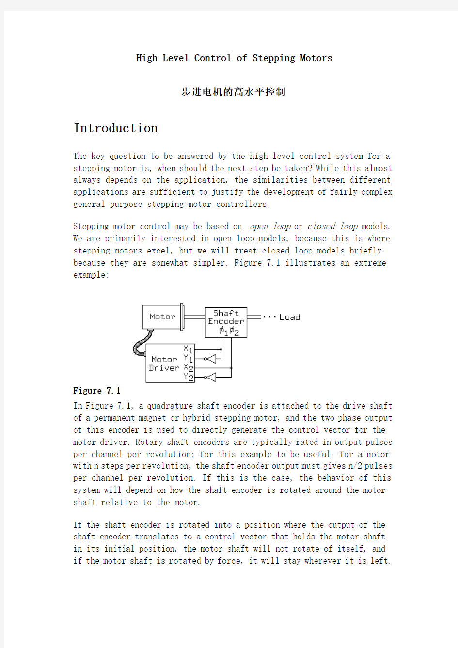
Stepping motor control may be based on open loop or closed loop models. We are primarily interested in open loop models, because this is where stepping motors excel, but we will treat closed loop models briefly because they are somewhat simpler. Figure 7.1 illustrates an extreme example:

Figure 7.1

In Figure 7.1, a quadrature shaft encoder is attached to the drive shaft of a permanent magnet or hybrid stepping motor, and the two phase output of this encoder is used to directly generate the control vector for the motor driver. Rotary shaft encoders are typically rated in output pulses per channel per revolution; for this example to be useful, for a motor with n steps per revolution, the shaft encoder output must gives n/2 pulses per channel per revolution. If this is the case, the behavior of this system will depend on how the shaft encoder is rotated around the motor shaft relative to the motor.

If the shaft encoder is rotated into a position where the output of the shaft encoder translates to a control vector that holds the motor shaft in its initial position, the motor shaft will not rotate of itself, and if the motor shaft is rotated by force, it will stay wherever it is left.

We will refer to this position of the shaft encoder relative to the motor as the neutral position.

If the shaft encoder is rotated one step clockwise (or counterclockwise) from the neutral position, the control vector output by the shaft encoder will pull the rotor clockwise (or counterclockwise). As the rotor turns, the shaft encoder will change the control vector so that the rotor is always trying to maintain a position one step clockwise (or counterclockwise) from where it is at the moment. The torque produced by this method will fall off with rotor speed, but this control system will always produce the maximum torque the motor is able to deliver at any speed.

In effect, with this one-step displacement, we have constructed a brushless DC motor from a stepping motor and a collection of off-the-shelf parts. In practice, this is rarely done, but there are numerous applications of stepping motors in closed-loop control systems that are based on this model, usually with a microprocessor included in the feedback loop between the shaft encoder and the motor controller.

In an open-loop control system, this feedback loop is broken, but at a high level, the basic principle remains quite similar, as illustrated in Figure 7.2:

Figure 7.2

In Figure 7.2, we replace the shaft encoder from Figure 7.1 with a simulation model of the response of the motor and load to the control vector. At any instant, the actual position of the rotor is unknown! Nonetheless, we can use the simulation model to predict, based on an assumed rotor position and velocity, how the motor will respond to the control vector, and we can construct this model so that its output is the control vector generated by a simulated shaft encoder.

So long as the model is sufficiently accurate, the behavior of the motor controlled by this model will be the same as the behavior of the motor controlled by a closed loop system!

Model Variables

In the example given in Figure 7.1, the only control variable offered is the angle of the shaft encoder relative to the motor. In effect, this controls the extent to which the equilibrium point of the motor's torque versus shaft angle curve leads or follows the current rotor position. In theory, any desired motor behavior can be elicited by adjusting this angle, but it is far more convenient to speak in terms of other variables:

-- The predicted shaft position (radians)

target -- The target shaft position determined by the application

V = d/dt -- The predicted velocity (radians per second)

V target -- The target velocity determined by the application

A = dV/dt -- The predicted acceleration (radians per second squared)

A target -- The target acceleration, may be determined by the application As in the section on Stepping Motor Physics, we will define the basic motor characteristics:

S -- step or microstep angle, in radians

μ -- moment of inertia of rotor and load

h -- the holding torque of the motor

Note that here, the step angle S is not the physical step angle of the motor, but rather, the step angle offered by the mid-level motor interface; this may be a full step, a half step, or a microstep of some size!

Models

The simplest model that will do the job is almost always the best. For some applications, this means the model is so simple that it is hard to identify it as a model! For example, consider the case where the application demands a constant motor velocity:

A target = 0

V target = Constant

In this case,

t step = S / V target

where

t step -- time per step

This barely looks like a model; in part, this is because we have omitted the statement that, every t step seconds, we advance the control vector one step:

repeat the following cycle forever:

wait t step seconds and then

= + S

step( 1 )

A more interesting model is required if we want to maintain a constant acceleration. Obviously, we can't do this forever, but we'll use this model as a component in more complex models that require changes of velocity or position. In this case,

A target = Constant

where

A target < h/ μ

In developing a model, we begin with the observation that, for constant acceleration A and assuming a standing start at time 0,

= 1/2 A t2

More generally, if the motor starts at position and velocity V, after time t the new position ' and velocity V' will be:

' = 1/2 A t2 + V t V' = A t + V

Setting =0 and '=S, we solve first for t, the time taken to move one step, as a function of V and A:

1/2 A t2 + V t - S = 0

t = ( -V ± ( V2 + 2 A S )0.5 ) / A

Here, we have applied the quadratic formula, and for our situation, this gives two real roots! The additive root is the root we are concerned with; for this, we can use the resulting time to compute the velocity at the end of one step:

t step = ( -V + ( V2 + 2 A S )0.5 ) / A

V' = ( V2 + 2 A S )0.5

We can combine this model for acceleration with the model for constant speed running to make a motor controller that will seek V target, assuming that an outside agent may change V target at any time:

repeat the following cycle forever:

if V = V target do the following:

wait S/V target seconds and then

= + S

step( 1 )

otherwise, if V < V target, accelerate as follows:

wait ( -V + (V2 + 2 A accel S)0.5 ) / A accel seconds and then

= + S

V = (V2 + 2 A accel S)0.5

step( 1 )

otherwise, V > V target, decelerate as follows:

wait ( -V + (V2 + 2 A decel S)0.5 ) / A decel seconds and then

= + S

V = (V2 + 2 A decel S)0.5

step( 1 )

This control system is not fully satisfactory for a number of reasons! First, it only allows the motor to operate in one direction and it fails utterly when V reaches zero; at that point, if a divide by zero operation is allowed to produce an infinite result, the program will wait infinitely and never again respond to change in the control input.

The second shortcoming of this program is simpler to correct: As written, there is an infinitesimal probability of the motor speed reaching the desired speed and staying there with V target equal to V. Far more likely, what will happen is that V will oscillate around V target, taking alternate accelerating and decelerating steps and never settling down at the desired running speed.

A quick and dirty solution to this latter problem is to add code to recognize when V passes V target during acceleration or deceleration; when this occurs, V can be set to V target. Formally, this is incorrect, but if the acceleration and deceleration rates are not too high and if there is sufficient damping in the system, this will work quite well.

In a frictionless system using sine-cosine microstepping at speeds below the cutoff speed for the motor, the available torque is effectively constant and we can use the full torque to accelerate or decelerate the motor, so the above control algorithm will work with

A accel = A decel = h/ μ

If there is significant static friction, we can take this into account as follows:

A accel = ( h - f) / μ

A decel = ( h + f) / μ

where

f -- frictional torque

If the motor is run using the maximum available acceleration and decleration, any unexpected increase in the load will cause the motor rotor to fall behind its predicted position, and the result will be a failure of the control system. As a result, open-loop stepping motor control systems are never run at the accelerations give above! In the case of full or half-stepping, where there is no sine-cosine torque compensation, the available torque varies over a range of a factor of 20.5, so we typically adjust the accelerations given above by this amount: A accel = ( ( h / 1.414 ) - f) / μ

A decel = ( ( h / 1.414 ) + f) / μ

If we operate consistently near the edge of the performance envelope, and if we never request a velocity V target near the resonant speed of the motor, we can safely accelerate through resonances without relying on damping. If, on the other hand, we select acceleration values that are significantly below the maximum that is possible, electrical or mechanical damping may be needed to avoid problems with resonance.

Note that it is not difficult to extend the above control model to account, at least approximately, for viscous friction and for the dropoff of torque as a function of speed. To do this, we merely modify the above formulas for A accel and A decel so that h and f are functions of V. Thus, instead of treating these as constants of the control algorithm, we must recompute the available acceleration at each step.

If our goal is to turn the motor smoothly from one set postion to another, we must first accelerate it, then perhaps coast at fixed speed for a while, then decelerate. The decision governing when to begin decelerating rests on a knowledge of the stopping distance from any particular velocity. Assuming that the available acceleration is constant over the relevant range of speeds, we can compute this from:

V = A decel t

= 1/2 A decel t2

First we solve for the stopping time,

t = V / A decel

and then we solve for the stopping angle

= 1/2 A decel ( V / A decel )2 = V2 / ( 2 A decel )

Given this, we can outline a procedure for moving the motor from its current estimated position to a step just beyond some target position: moveto( target )

-- a function of one argument

-- no value is returned

while V < V target

and while < target - V2 / ( 2 A decel ) repeat the following to

accelerate

step( 1 )

wait ( -V + (V2 + 2 A accel S)0.5 ) / A accel seconds and then

= + S

V = (V2 + 2 A accel S)0.5

V = V target

while < target - V2 / ( 2 A decel ) repeat the following to coast

step( 1 )

wait S/V target seconds and then

= + S

while < target repeat the following to decelerate

step( 1 )

wait ( -V + ( V2 + 2 A decel S )0.5 ) / A accel seconds and then

= + S

V = ( V2 + 2 A accel S )0.5

V = 0

done, and target are within a step of each other!

The control model only moves the motor one direction, it fails to plan in terms of the quantization of available stopping positions, and it

doesn't account for the cyclic nature of . Nonetheless, it is a useful illustration. Note that we have used V target as a limiting velocity in this code, but that this will only be relevant during long moves; for short moves, the motor will never reach this speed.

With the above, code, so long as the acceleration and deceleration rates are high enough to avoid dwelling for too long at resonant speeds, and so long as V target is not too close to a resonant speed, a plot of rotor position versus time will show fairly clean moves, as illustrated in Figure 7.3:

Figure 7.3

If the motor is to be accelerated at the maximum possible rate, the control model used above is not sufficient. In that case, during acceleration, the equilibrium position must be maintained between 0.5 and 1.5 steps ahead of the rotor position as the rotor moves, and during deceleration, the equilibrium position must be maintained the same distance behind the rotor position. This requires careful logic at the turnaround point, when the change is made from accelerating to decelerating modes. The above control model omits any such considerations, but it is adequate at accelerations sufficiently below the maximum available!

Hardware Solutions

Today, it is rare to find high-level stepping motor control done purely in hardware, and when it is done, it is usually only in the very simplest of applications. For example, consider the problem of starting and stopping a stepping motor under load. Direct generation of the quadratic functions necessary to achieve smooth acceleration is quite difficult in hardware, but it is easy to generate exponentials that are adequate approximations of these. The circuit outlined in Figure 7.4 illustrates how this can be done:

Figure 7.4

Here, the resistor R and capacitor C form a low pass filter on the control input of the voltage controlled oscillator VCO. When the input level is at run, the VCO output oscillates at its maximum rate. When the input level is at stop, the VCO output ceases to oscillate. The RC time constant of

the low pass filter determines the rate of acceleration applied to the motor.

With such a design, the time constant RC is usually determined empirically by setting up the system and then adjusting R and C until the system operates properly.

Practical Examples

The NE555 timer can be used as a voltage controlled oscillator, but I first saw this done with discrete components on a controller for a paper-tape reader designed around 1970.

Software Solutions

The basic control models outlined at the start of this section can be directly incorporated into the software for controlling a stepping motor, and this must be done if, for example, the motor is driving a load with a variable moment of inertia or driving a load against variable frictional loadings. Most open-loop stepping motor applications are not that complicated, however! So long as the inertia and frictional loadings are constant, the control software can be greatly simplified, replacing complex model computations with a table of precomputed delays.

Consider the problem of accelerating the motor from a standing start. No matter where the motor starts, so long as the torque, moment of inertia and frictional loadings remain the same, the time sequence of steps will be the same. Therefore, we need only pre-compute this time sequence of steps and save it in an array. We can use this array as follows to accelerate the motor:

array AV, the acceleration vector, holds time intervals

i is the index into AV

i = 0

repeat the following cycle to accelerate forever:

wait AV[i] seconds and then

step( 1 )

i = i + 1

We may use i, the counter in the above code, as a stand-in for the motor velocity, since stepping the motor every AV[i] seconds will move the motor at a speed of S/AV[i].

It is a straightforward exercise in elementary physics to compute the entries in the array A. If the motor is accelerating at A target,

i = 1/2 A target t i 2

where

i -- the shaft angle at each successive step

Solving for time as a function of position, we get:

t i = (2i / A target) 0.5

If we define

0 = 0

so that

i = Si

and

t0 = 0

we can conclude that

t i = k i0.5

where

k = (2S/A target)0.5

The acceleration vector entries are then:

A[0] = (2S/A target)0.5

and

A[i] = (i0.5 - (i - 1)0.5)A[0]

The following table gives the ratios of the first 20 entries in A[i] to

In general, we aren't interested in indefinite acceleration, but rather, we are interested in accelerating until some speed or position restriction is satisfied, and then the control system should change, for example, from acceleration to deceleration or constant speed operation. So long as friction can be ignored, so the same rates can be used for acceleration and deceleration, we can make a clean move to a target position as follows:

array AV is the acceleration vector

i is the index into AV

i = 0

D = target -

while D nonzero do the following

if D > 0 -- spin one way

step( 1 )

D = D - 1

else -- spin the other way

step( -1 )

D = D + 1

endif

wait AV[i] seconds and then

if (i < |D|) and (S/AV[i] < V target) -- accelerate

i = i + 1

else if i > |D| -- decelerate

i = i - 1

endif

endloop

Given an appropriate acceleration vector, the above code will cleanly accelerate a motor up to a speed near the target velocity, hold that speed, and then decelerate cleanly to a stop at the target position.

The above code does not take advantage of the higher rates of deceleration allowed when there is friction. In general, this should not cause any problems, but if the fastest possible moves are desired, a separate deceleration table should be maintained. Here is one idea:

array AV holds acceleration intervals

array C holds coasting intervals

array T holds transition information

array D holds deceleration intervals

i = 0

repeat the following until the desired speed is reached

wait A[i] seconds and then

step( 1 )

i = i + 1

repeat the following to maintain the speed

wait C[i] seconds and then

step( 1 )

repeat the following to maintain the speed

i = i - T[i]

repeat the following until i = 0

i = i - 1

step( 1 )

In the above, the arrays A and D are constructed identically, except that one has intervals used for acceleration, at a rate limited by friction, while the other has intervals used for deceleration, at a rate assisted by friction. Note that, after accelerating for i steps from a standing start, the motor will reach a velocity from which it can decelerate to a halt in i-T[i] steps. This relationship determines the values pre-computed in the array T.

usb驱动程序教程

编写Windows https://www.wendangku.net/doc/6a8686798.html,的usb驱动程序教程 Windows https://www.wendangku.net/doc/6a8686798.html, 是微软推出的功能强大的嵌入式操作系统，国内采用此操作系统的厂商已经很多了，本文就以windows https://www.wendangku.net/doc/6a8686798.html,为例，简单介绍一下如何开发windows https://www.wendangku.net/doc/6a8686798.html, 下的USB驱动程序。 Windows https://www.wendangku.net/doc/6a8686798.html, 的USB系统软件分为两层： USB Client设备驱动程序和底层的Windows CE实现的函数层。USB设备驱动程序主要负责利用系统提供的底层接口配置设备，和设备进行通讯。底层的函数提本身又由两部分组成，通用串行总线驱动程序（USBD）模块和较低的主控制器驱动程序（HCD）模块。HCD负责最最底层的处理，USBD模块实现较高的USBD函数接口。USB设备驱动主要利用 USBD接口函数和他们的外围设备打交道。 USB设备驱动程序主要和USBD打交道，所以我们必须详细的了解USBD提供的函数。主要的传输函数有： abourttransfer issuecontroltransfer closetransfer issuein te rruptransfer getisochresult issueisochtransfer gettransferstatus istransfercomplete issuebulktransfer issuevendortransfer 主要的用于打开和关闭usbd和usb设备之间的通信通道的函数有： abortpipetransfers closepipe isdefaultpipehalted ispipehalted openpipe resetdefaultpipe resetpipe 相应的打包函数接口有： getframelength getframenumber releaseframelengthcontrol setframelength takeframelengthcontrol 取得设置设备配置函数： clearfeature setdescriptor getdescriptor setfeature

USB驱动程序编写

USB驱动程序编写 linux下usb驱动编写（内核2.4）——2.6与此接口有区别2006-09-15 14:57我们知道了在Linux 下如何去使用一些最常见的USB设备。但对于做系统设计的程序员来说，这是远远不够的，我们还需要具有驱动程序的阅读、修改和开发能力。在此下篇中，就是要通过简单的USB驱动的例子，随您一起进入USB驱动开发的世界。 USB骨架程序（usb-skeleton），是USB驱动程序的基础，通过对它源码的学习和理解，可以使我们迅速地了解USB驱动架构，迅速地开发我们自己的USB硬件的驱动。 USB驱动开发在掌握了USB设备的配置后，对于程序员，我们就可以尝试进行一些简单的USB驱动的修改和开发了。这一段落，我们会讲解一个最基础USB框架的基础上，做两个小的USB驱动的例子。 USB骨架在Linux kernel源码目录中driver/usb/usb-skeleton.c为我们提供了一个最基础的USB驱动程序。我们称为USB骨架。通过它我们仅需要修改极少的部分，就可以完成一个USB设备的驱动。我们的USB驱动开发也是从她开始的。那些linux下不支持的USB设备几乎都是生产厂商特定的产品。如果生产厂商在他们的产品中使用自己定义的协议，他们就需要为此设备创建特定的驱动程序。当然我们知道，有些生产厂商公开他们的USB协议，并帮助Linux驱动程序的开发，然而有些生产厂商却根本不公开他们的USB协议。因为每一个不同的协议都会产生一个新的驱动程序，所以就有了这个通用的USB驱动骨架程序，它是以pci 骨架为模板的。如果你准备写一个linux驱动程序，首先要熟悉USB协议规范。USB主页上有它的帮助。一些比较典型的驱动可以在上面发现，同时还介绍了USB urbs的概念，而这个是usb驱动程序中最基本的。 Linux USB 驱动程序需要做的第一件事情就是在Linux USB 子系统里注册，并提供一些相关信息，例如这个驱动程序支持那种设备，当被支持的设备从系统插入或拔出时，会有哪些动作。所有这些信息都传送到USB 子系统中，在usb骨架驱动程序中是这样来表示的： static struct usb_driver skel_driver = { name: skeleton, probe: skel_probe, disconnect: skel_disconnect, fops: &skel_fops, minor: USB_SKEL_MINOR_BASE, id_table: skel_table,

USB设备驱动程序设计

USB设备驱动程序设计引言 USB 总线是1995 年微软、IBM 等公司推出的一种新型通信标准总线，特点是速度快、价格低、独立供电、支持热插拔等，其版本从早期的1.0、1.1 已经发展到目前的2.0 版本，2.0 版本的最高数据传输速度达到480Mbit/s，能满足包括视频在内的多种高速外部设备的数据传输要求，由于其众多的优点，USB 总线越来越多的被应用到计算机与外设的接口中，芯片厂家也提供了多种USB 接口芯片供设计者使用，为了开发出功能强大的USB 设备，设计者往往需要自己开发USB 设备驱动程序，驱动程序开发一直是Windows 开发中较难的一个方面，但是通过使用专门的驱动程序开发包能减小开发的难度，提高工作效率，本文使用Compuware Numega 公司的DriverStudio3.2 开发包，开发了基于NXP 公司USB2.0 控制芯片ISP1581 的USB 设备驱动程序。 USB 设备驱动程序的模型 USB 设备驱动程序是一种典型的WDM(Windows Driver Model)驱动程序，其程序模型如图1 所示。用户应用程序工作在Windows 操作系统的用户模式层，它不能直接访问USB 设备，当需要访问时，通过调用操作系统的 API(Application programming interface)函数生成I/O 请求信息包(IRP)，IRP 被传输到工作于内核模式层的设备驱动程序，并通过驱动程序完成与UBS 外设通信。设备驱动程序包括两层：函数驱动程序层和总线驱动程序层，函数驱动程序一方面通过IRP 及API 函数与应用程序通信，另一方面调用相应的总线驱动程序，总线驱动程序完成和外设硬件通信。USB 总线驱动程序已经由操作系统提供，驱动程序开发的重点是函数驱动程序。 USB 设备驱动程序的设计

开发usb驱动程序的方法(连载一)

开发usb驱动程序的方法（连载一）开始驱动程序设计下面的文字是从Microsoft的DDK帮助中节选出来的，它让我们明白在开始设计驱动程序应该注意些什么问题，这些都是具有普遍意义的开发准则。应该支持哪些I/O请求在开始写任何代码之前，应该首先确定我们的驱动程序应该处理哪些IRP例程。如果你在设计一个设备驱动程序，你应该支持和其他相同类型设备的NT驱动程序相同的IRP_MJ_XXX 和IOCTL请求代码。如果你是在设计一个中间层NT驱动程序，应该首先确认你下层驱动程序所管理的设备，因为一个高层的驱动程序必须具有低层驱动程序绝大多数IRP_MJ_XXX例程入口。高层驱动程序在接到I/O 请求时，在确定自身IRP当前堆栈单元参数有效的前提下，设置好IRP中下一个低层驱动程序的堆栈单元，然后再调用IoCallDriver 将请求传递给下层驱动程序处理。一旦决定好了你的驱动程序应该处理哪些IRP_MJ_XXX，就可以开始确定驱动程序应该有多少个Dispatch例程。当然也可以考虑把某些 RP_MJ_XXX处理的例程合并为同一例程处理。例如在ChangerDisk 和 VDisk里，对IRP_MJ_CREATE和IRP_MJ_CLOSE处理的例程就是同一函数。对IRP_MJ_READ和IRP_MJ_WRITE处理的例程也是同一个函数。应该有多少个Device对象？一个驱动程序必须为它所管理的每个可能成为I/O请求的目标的物理和逻辑设备创建一个命名Device对象。一些低层的驱动程序还可能要创建一些不确定数目的Device对象。例如一个硬盘驱动程序必须为每一个物理硬盘创建一个Device对象，同时还必须为每个物理磁盘上的每个逻辑分区创建一个Device对象。一个高层驱动驱动程序必须为它所代表的虚拟设备创建一个Device 对象，这样更高层的驱动程序才能连接它们的Device对象到这个驱动程序的Device对象。另外，一个高层驱动程序通常为它低层驱动程序所创建的Device对象创建一系列的虚拟或逻辑Device对象。尽管你可以分阶段来设计你的驱动程序，因此一个处在开发阶段的驱动程序不必一开始就创建出所有它将要处理的所有Device对象。但从一开始就确定好你最终要创建的所有Device对象将有助于设计者所要解决的任何同步问题。另外，确定所要创建的Device对象还有助于你定义Device对象的Device Extension 的内容和数据结构。开始驱动程序开发驱动程序的开发是一个从粗到细逐步求精的过程。NT DDK的src\ 目录下有一个庞大的样板代码，几乎覆盖了所有类型的设备驱动程序、高层驱动程序和过滤器驱动程序。在开始开发你的驱动程序之前，你应该在这个样板库下面寻找是否有和你所要开发的类似类型的例程。例如我们所开发的驱动程序，虽然DDK 对USB描述得不是很详细，我们还是可以在src\storage\class目录发现很多和USB设备有关的驱动程序。下面我们来看开发驱动程序的基本步骤。最简的驱动程序框架 1、写一个DriverEntry例程，在里面调用IoCreateDevice创建一个Device对象。 2、写一个处理IRP_MJ_CREA TE请求的Dispatch例程的基本框架 (参见DDK Kernel-Mode Drivers 4.4.3描述的一个DispatchCreate 例程所要完成的最基本工作。当然写了DispatchCreate例程后，要在DriverEntry 例程为IRP_MJ_CREA TE初始化例程入口)。如果驱动程序创建了多于一个Device对象，则必须为IRP_MJ_CLOSE 请求写一个例程，该例程通常情况下可以和DispatchCreate共用一个例程，参见参见DDK Kernel-Mode Drivers 4.4.3。 3、编译连接你的驱动程序。

USB驱动程序的编写采用WDM驱动程序

U S B驱动程序的编写采用W D M驱动程序 Document serial number【UU89WT-UU98YT-UU8CB-UUUT-UUT108】

USB驱动程序的编写采用WDM 驱动程序。WDM 驱动程序是一些例程的集合，它们被动地存在，等待主机系统软件（PnP 管理器、I/O 管理器、电源管理器等）来调用或激活它们。具体驱动程序不同，其所包含的例程也不同。一个WDM 驱动程序的基本组成包括以下5个例程：（1）驱动程序入口例程：处理驱动程序的初始化。（2）即插即用例程：处理PnP 设备的添加、删除和停止。（3）分发例程：处理用户应用程序发出的各种 I/O 请求。（4）电源管理例程：处理电源管理请求。（5）卸载例程：处理驱动程序的卸载。包含文件： , , , , , makefile,sources) 在文件中，包含了上述五个例程：中定义了各种数据结构还有各种IOCTL控制码，用于不同数据的读写。

中实现了各种驱动例程。包含了上述五个所说例程外还包含了其他例程，课程从下面的驱动程序入口例程得出一些信息。驱动程序入口例程： NTSTATUS DriverEntry( IN PDRIVER_OBJECT DriverObject, IN PUNICODE_STRING RegistryPath ) { NTSTATUS ntStatus = STATUS_SUCCESS; PDEVICE_OBJECT deviceObject = NULL; DriverObject->MajorFunction[IRP_MJ_CREATE] = Ezusb_Create; DriverObject->MajorFunction[IRP_MJ_CLOSE] = Ezusb_Close; ources. If you want to add a new source # file to this

编写USB驱动程序步骤

编写USB驱动程序步骤： 1所有usb驱动都必须创建主要结构体struct usb_driver struct usb_driver ->struct module *owner (有他可正确对该驱动程序引用计数，应为THIS_MODULE） ->const char *name (驱动名字，运行时可在查看 /sys/bus/usb/drivers/) ->const struct usb_device_id *id_table (包含该驱动可支持的所有不同类型的驱动设备,没添探测回调函数不会被调用） ->int （*probe)(struct usb_interface *intf,const struct usb_device_id *id) (usb驱动探测函数,确认后struct usb_interface 应恰当初始化，然后返0，如果出错则返负值) ->void(*disconnect)(struct usb_interface *intf) (当struct usb_interface 被从系统中移除或驱动正从usb核心中卸载时，usb核心将调用此函数）代码实例： static struct usb_driver skel_driver={ .owner = THIS_MODULE, .name = "skeleton", .id_table = skel_table, .probe = skel_probe, .disconnect = skel_disconnect, }; ↓ 2usb_register()注册将struct usb_driver 注册到usb核心，传统是在usb驱动程序模块初始化代码中完成该工作的

USB键盘驱动程序

/* * $Id: usbkbd.c,v 1.27 2001/12/27 10:37:41 vojtech Exp $ * * Copyright (c) 1999-2001 Vojtech Pavlik * * USB HIDBP Keyboard support */ /* * This program is free software; you can redistribute it and/or modify * it under the terms of the GNU General Public License as published by * the Free Software Foundation; either version 2 of the License, or * (at your option) any later version. * * This program is distributed in the hope that it will be useful, * but WITHOUT ANY WARRANTY; without even the implied warranty of * MERCHANTABILITY or FITNESS FOR A PARTICULAR PURPOSE. See the * GNU General Public License for more details. * * You should have received a copy of the GNU General Public License * along with this program; if not, write to the Free Software * Foundation, Inc., 59 Temple Place, Suite 330, Boston, MA 02111-1307 USA * * Should you need to contact me, the author, you can do so either by * e-mail - mail your message to , or by paper mail: * Vojtech Pavlik, Simunkova 1594, Prague 8, 182 00 Czech Republic */ #include #include #include #include #include #include #include /* * Version Information */ #define DRIVER_VERSION "" #define DRIVER_AUTHOR "Vojtech Pavlik " #define DRIVER_DESC "USB HID Boot Protocol keyboard driver" #define DRIVER_LICENSE "GPL"

USB驱动编程指南

USB驱动编写指南 1 概念：模块和设备文件 1.1模块模块是在核空间运行的程序，实际上是一种目标对象文件，没有，不能独立运行，但是可以装载到系统中作为核的一部分运行，从而可以动态扩充核的功能。模块最主要的用处就是用来实现设备驱动程序。Linux下对于一个硬件的驱动，可以有两种方式：直接加载到核代码中，启动核时就会驱动此硬件设备。另一种就是以模块方式，编译生成一个.ko文件(在2.4以下核中是用.o作模块文件，我们以2.6的核为准，以下同)。当应用程序需要时再加载到核空间运行。所以我们所说的一个硬件的驱动程序，通常指的就是一个驱动模块。 1.2设备文件设备文件对于一个设备，它可以在/dev下面存在一个对应的逻辑设备节点，这个节点以文件的形式存在，但它不是普通意义上的文件，它是设备文件，更确切的说，它是设备节点。这个节点是通过mknod命令建立的，其中指定了主设备号和次设备号。主设备号表明了某一类设备，一般对应着确定的驱动程序；次设备号一般是区分不同属性，例如不同的使用方法，不同的位置，不同的操作。这个设备号是从/proc/devices文件中获得的，所以一般是先有驱动程序在核中，才有设备节点在目录中。这个设备号（特指主设备号）的主要作用，就是声明设备所使用的驱动程序。驱动程序和设备号是一一对应的，当你打开一个设备文件时，操作系统就已经知道这个设备所对应的驱动程序。对于一个硬件，Linux是这样来进行驱动的：首先，我们必须提供一个.ko的驱动模块文件。我们要使用这个驱动程序，首先要加载它，我们可以用insmod xxx.ko，这样驱动就会根据自己的类型（字符设备类型或块设备类型，例如鼠标就是字符设备而硬盘就是块设备）向系统注册，注册成功系统会反馈一个主设备号，这个主设备号就是系统对它的唯一标识。驱动就是根据此主设备号来创建一个一般放置在/dev目录下的设备文件。在我们要访问此硬件时，就可以对设备文件通过open、read、write、close等命令进行。而驱动就会接收到相应的read、write操作而根据自己的模块中的相应函数进行操作了。 2 USB驱动程序如何应用了解了上述理论后，我们就可以动手写驱动程序，如果你基本功好，而且写过linux下的硬件驱动，USB的硬件驱动和pci_driver很类似，那么写USB的驱动就比较简单了，如果你只是大体了解了linux的硬件驱动，那也不要紧，因为在linux的核源码中有一个框架程序可以拿来借用一下，这个框架程序在/usr/src/~（你的核版本，以下同）/drivers/usb下，文件名为usb-skeleton.c。写一个USB的驱动程序最基本的要做四件事：驱动程序要支持的设备、注册USB驱动程序、探测和断开、提交和控制urb（USB请求块）（当然也可以不用urb 来传输数据，下文我们会说到）。 2.1驱动程序支持的设备驱动程序支持的设备有一个结构体struct usb_device_id，这个结构体提供了一列不同类型的该驱动程序支持的USB设备，对于一个只控制一个特定的USB设备的驱动程序来说，struct usb_device_id表被定义为： /* 驱动程序支持的设备列表*/ static struct usb_device_id skel_table = { { USB_DEVICE(USB_SKEL_VENDOR_ID, USB_SKEL_PRODUCT_ID) },

USB驱动程序编写和安装导入

10分钟完成一个USB驱动程序很多写Windows Device Driver的开发人员基本上都是使用Windows DDK进行开发的。但是，现在也有不少人都开始借助一些辅助工具。笔者去年开始接触到riverStudio，发现它真的是一个不错的开发工具，不仅写代码的时候思路清晰，而且和DDK的结合很好。当然，也有很多人觉得用DriverStudio不够正宗，或者说不能很好的理解Windows Device Driver的架构。我感觉这就有点像MFC和SDK的关系，关于这个问题在很多地方都有争论，比如在万千新闻组上，就讨论了将近2个月。每个人都有自己的最爱，都有自己的习惯，只要你能把事情做好，我想用什么方法应该都是一样的。如果你已经习惯了用DDK开发，那完全还可以继续用下去；如果你觉得DriverStudio不错，那尝试用一个可以给你按照OOP概念来编程的工具有什么不好呢？在驱动开发网上，经常看到有人询问一些关于DriverStudio的使用的问题。我正好很有幸用它作了几个驱动程序，包括VXD, KMD和WDM，稍微有点心得，因此想写下来给大家作一个小小的参考。如果其中有错误，欢迎大家给我指出，谢谢。下面我就介绍一下用DriverStudio开发一个USB驱动程序的过程。这个USB设备有3个双向端点，每个端点的配置如下： EP 类型地址buffer(Bytes) 0 IN/OUT Control 0x80/0x00 16/16 1 IN/OUT Bulk 0x81/0x01 16/16 2 IN/OUT Bulk 0x82/0x02 64/64 我们的驱动程序需要实现的功能就是控制设备上的LED灯的亮和灭，以及通过Endpoint 2对设备进行读写。由于DriveStudio由几个部分组成，我们写这个驱动程序只要用到DriverWorks，因此下面我们就简称它为DW。在这里，我们假定读者已经正确的安装了DW，并且已经编译好了各个库文件。 1. 首先，我们通过快捷方式“Setup DDK and Start MSVC“来启动VC IDE。这个快捷方式所指向的程序，会进行一些必要的设置，然后再启动VC IDE，这样我们的程序就可以使用DDK和DW的头文件和库了。 2. 从VC IDE的菜单"DriverStudio"中选择"DriverWizard", 在如图1所示的对话框中, 写上项目名称. 在这里, 我们将这个项目称为: TEST, 所在的目录为D:\TEST. 然后点按钮"Next >".

usb驱动程序的编写采用wdm驱动程序

驱动程序入口例程： NTSTATUS DriverEntry( IN PDRIVER_OBJECT DriverObject, IN PUNICODE_STRING RegistryPath ) { NTSTATUS ntStatus = STATUS_SUCCESS; PDEVICE_OBJECT deviceObject = NULL; DriverObject->MajorFunction[IRP_MJ_CREATE] = Ezusb_Create; DriverObject->MajorFunction[IRP_MJ_CLOSE] = Ezusb_Close; ources. If you want to add a new source # file to this component. This file merely indirects to the real make file # that is shared by all the driver components of the Windows NT DDK # !INCLUDE $(NTMAKEENV) 不要编辑这个文件。事实上每个WDM程序所需要的makefile的内容都是一样的，只需要简单地copy 一个makefile到新的项目中就可以了

开发usb驱动程序的方法

开发驱动程序的方法（连载一）开始驱动程序设计下面的文字是从的帮助中节选出来的，它让我们明白在开始设计驱动程序应该注意些什么问题，这些都是具有普遍意义的开发准则。应该支持哪些请求在开始写任何代码之前，应该首先确定我们的驱动程序应该处理哪些例程。如果你在设计一个设备驱动程序，你应该支持和其他相同类型设备的驱动程序相同的和请求代码。如果你是在设计一个中间层驱动程序，应该首先确认你下层驱动程序所管理的设备，因为一个高层的驱动程序必须具有低层驱动程序绝大多数例程入口。高层驱动程序在接到请求时，在确定自身当前堆栈单元参数有效的前提下，设置好中下一个低层驱动程序的堆栈单元，然后再调用将请求传递给下层驱动程序处理。一旦决定好了你的驱动程序应该处理哪些，就可以开始确定驱动程序应该有多少个例程。当然也可以考虑把某些处理的例程合并为同一例程处理。例如在和里，对和处理的例程就是同一函数。对和处理的例程也是同一个函数。应该有多少个对象？一个驱动程序必须为它所管理的每个可能成为请求的目标的物理和逻辑设备创建一个命名对象。一些低层的驱动程序还可能要创建一些不确定数目的对象。例如一个硬盘驱动程序必须为每一个物理硬盘创建一个对象，同时还必须为每个物理磁盘上的每个逻辑分区创建一个对象。一个高层驱动驱动程序必须为它所代表的虚拟设备创建一个对象，这样更高层的驱动程序才能连接它们的对象到这个驱动程序的对象。另外，一个高层驱动程序通常为它低层驱动程序所创建的对象创建一系列的虚拟或逻辑对象。尽管你可以分阶段来设计你的驱动程序，因此一个处在开发阶段的驱动程序不必一开始就创建出所有它将要处理的所有对象。但从一开始就确定好你最终要创建的所有对象将有助于设计者所要解决的任何同步问题。另外，确定所要创建的对象还有助于你定义对象的的内容和数据结构。开始驱动程序开发驱动程序的开发是一个从粗到细逐步求精的过程。的\ 目录下有一个庞大的样板代码，几乎覆盖了所有类型的设备驱动程序、高层驱动程序和过滤器驱动程序。在开始开发你的驱动程序之前，你应该在这个样板库下面寻找是否有和你所要开发的类似类型的例程。例如我们所开发的驱动程序，虽然对描述得不是很详细，我们还是可以在\\目录发现很多和设备有关的驱动程序。下面我们来看开发驱动程序的基本步骤。最简的驱动程序框架、写一个例程，在里面调用创建一个对象。、写一个处理请求的例程的基本框架 (参见 4.4.3描述的一个例程所要完成的最基本工作。当然写了例程后，要在例程为初始化例程入口)。如果驱动程序创建了多于一个对象，则必须为请求写一个例程，该例程通常情况下可以和共用一个例程，参见参见。、编译连接你的驱动程序。用下面的方法来测试你的驱动程序。首先按上面介绍的方法安装好驱动程序。其次我们还得为逻辑设备名称和目标对象名称之间建立起符号连接，我们在前面已经知道对象名称对用户模式是不可见的，是不能直接通过来访问的，只能访问逻辑设备名称。我们可以通过修改注册表来建立这两种名称之间的符号连接。运行在\\ \ \\ \ 下建立起符号连接(这种符号连接也可以在驱动程序里调用函数来创建）。

(简易USB驱动)开发指导

实验七（2）设备驱动开发指导块设备种类多，使用广泛，其驱动程序的开发也比字符设备复杂。通过本实验，大家要开发一个实际块设备（U盘）的驱动程序，将能够更深入地掌握块设备驱动程序的开发方法。Linux下已经有一个通用的U盘驱动程序usb-storage.o，其源程序放在目录drivers\usb\storage下（相对于内核源码根目录）。但这个驱动的实现相当复杂，本实验希望开发一个相对简单些的U盘驱动程序，不求高性能，只求结构明朗、清晰易懂，主要是让大家掌握一个实际块设备的驱动方式，从而加深理解。事实上，本实验开发的驱动程序应该能够适用于所有基于Bulkonly传输协议的USB大容量存储设备（USB Mass Storage），比如USB移动硬盘和USB外置光驱，USB闪存盘（U 盘）只是其中的一种。由于USB大容量存储设备具有容量大、速度快、连接灵活、即插即用、总线供电等优点，它们得到了广泛使用，掌握这类设备驱动程序的开发技术无疑具有很强的实用性。实验内容编写一个U盘驱动程序myudisk，只要求能够驱动某个型号的U盘，能够支持U盘的常规操作，如命令hexdump、mke2fs和mount等。同时，要求在系统内核日志中显示出U盘的容量。若有余力，可增加多分区支持功能。实验基础和思路在教材中P130，讲解了如何编写一个Ramdisk块设备驱动程序(sbull.c)，称为radimo；在文献《Linux Device Drivers》讲解了如何编写一个USB设备驱动程序，并以Linux源代码中的usb-skeleton.c为例。虽然前者驱动的并不是一个实际的块设备，且后者又只是针对usb字符设备，但是它们提供了一个不错的基础，通过合并我们就能基本得到一个支持usb块设备的驱动程序。之所以说基本得到，是因为合并后只是有了块设备、USB设备的驱动支持框架，但还缺一样：对U盘（USB块设备）的实际访问操作。USB块设备的访问方法与USB字符设备区别很大，有一套复杂的协议。把这样一套协议研究清楚，将花费大量时间，也远离了我们驱动程序开发的核心。这是一大难点，为此我们专门编写了一个U盘访问函数（myudisk_Bulk_transport），以减轻工作量。下一节将对该函数的使用方法和工作过程进行专门讲解。简言之，合并radimo和usb-skeleton这两个参考驱动程序，以构造整体框架，调用帮助函数myudisk_Bulk_transport以访问U盘，从而打造一个简洁的U盘驱动程序。本节接下来介绍这两个参考驱动程序：radimo和usb-skeleton，着重讲解其工作原理及合并关键环节。参考驱动程序一：块设备驱动程序sbull 请参看教材P130

USB上位机驱动程序环境搭建

USB上位机驱动程序环境搭建（一）WinXP SP1+DS3.2+XP DDK+VC6.0 分享修改我使用的是WinXP SP2+DS3.2+XP DDK+VC6.0英文版，以下为DS3.2版本的安装过程： 1.安装英文原版Visual studio 6.0，同时要记住注册环境变量。 2.安装XPDDK，安装时候注意需要将所有的组件、工具、例子等都安装（避免出现头文件和链接库找不到的问题）； 3.安装DS3.2； 4.通过DriverStudio菜单{C:\Documents and Settings\All Users\「开始」菜单\程序\Compuware DriverStudio\Develop}下的DDK Build Settings子菜单启动VC,不要去点桌面上的快捷方式。 5.用Open Workspace打开位于DS安装目录的 ……\DriverWorks\Source\vdwlibs.dsw。 6. 选择VC的Build菜单，选择batch Build，在之后的对话框中选择"Select x86",然后点击Rebuld all.等待编译成功,编译成功后， vdw_wdm.lib会在{E:\Program Files\Compuware\DriverStudio\DriverWorks\lib\i386\checked（或是free）}下。 7. 打开位于……\DriverWorks\Examples\wdm\hellowdm.dsw，然后编译（用VC的编译和用DS增加的编译钮都可以）。如果你可以在其目录中找到hellowdm.sys你就成功了。如果程序报警：不能找到kcsq.h，可到{E:\Program

USB驱动开发(一)

一USB的框架提到USB的框架，先看一张很经典的架构图总结一句话就是：设备通常有一个或多个配置，配置通常有一个或多个接口，接口通常有一个或多个设置，接口有零或多个端点。设备描述符是用来记录设备的通用信息，比如供应商ID、产品ID和修订ID，支持的设备类、子类和适用的协议以及默认端点的最大包大小等 struct usb_device_descriptor { _ _u8 bLength; //描述符长度 _ _u8 bDescriptorType; //描述符类型编号 _ _le16 bcdUSB; //USB版本号 _ _u8 bDeviceClass; //USB分配的设备类code _ _u8 bDeviceSubClass; // USB分配的子类code _ _u8 bDeviceProtocol; //USB分配的协议code _ _u8 bMaxPacketSize0; //endpoint0最大包大小 _ _le16 idVendor; //厂商编号 _ _le16 idProduct; //产品编号 _ _le16 bcdDevice; //设备出厂编号 _ _u8 iManufacturer; //描述厂商字符串的索引 _ _u8 iProduct; //描述产品字符串的索引 _ _u8 iSerialNumber; //描述设备序列号字符串的索引 _ _u8 bNumConfigurations; //可能的配置数量 } _ _attribute_ _ ((packed)); 配置描述符可以包含一个或多个配置，比如USB设备的低功耗模式和高功耗模式可分别对应一个配置。但是存在多个配置时，在使用USB设备前，必须为其选择一个合适的配置。USB设备的每一个配置都必须有一个配置描述符。 struct usb_config_descriptor { _ _u8 bLength; //描述符长度 _ _u8 bDescriptorType; //描述符类型编号 _ _le16 wTotalLength; //配置所返回的所有数据的大小 _ _u8 bNumInterfaces; // 配置所支持的接口数

studio10分钟完成一个USB驱动程序

10分钟完成一个USB驱动程序 (Rayyang2000倾情奉献) 很多写Windows Device Driver的开发人员基本上都是使用Windows DDK进行开发的。但是，现在也有不少人都开始借助一些辅助工具。笔者去年开始接触到driverStudio，发现它真的是一个不错的开发工具，不仅写代码的时候思路清晰，而且和DDK的结合很好。当然，也有很多人觉得用DriverStudio不够正宗，或者说不能很好的理解Windows Device Driver的架构。我感觉这就有点像MFC和SDK的关系，关于这个问题在很多地方都有争论，比如在万千新闻组上，就讨论了将近2个月。每个人都有自己的最爱，都有自己的习惯，只要你能把事情做好，我想用什么方法应该都是一样的。如果你已经习惯了用DDK开发，那完全还可以继续用下去；如果你觉得DriverStudio不错，那尝试用一个可以给你按照OOP概念来编程的工具有什么不好呢？在驱动开发网上，经常看到有人询问一些关于DriverStudio的使用的问题。我正好很有幸用它作了几个驱动程序，包括VXD, KMD和WDM，稍微有点心得，因此想写下来给大家作一个小小的参考。如果其中有错误，欢迎大家给我指出，谢谢。下面我就介绍一下用DriverStudio开发一个USB驱动程序的过程。这个USB设备有3个双向端点，每个端点的配置如下： EP 类型地址 buffer(Bytes) 0 IN/OUT Control 0x80/0x00 16/16 1 IN/OUT Bulk 0x81/0x01 16/16 2 IN/OUT Bulk 0x82/0x02 64/64 我们的驱动程序需要实现的功能就是控制设备上的LED灯的亮和灭，以及通过Endpoint 2对设备进行读写。由于DriveStudio由几个部分组成，我们写这个驱动程序只要用到DriverWorks，因此下面我们就简称它为DW。在这里，我们假定读者已经正确的安装了DW，并且已经编译好了各个库文件。 1. 首先，我们通过快捷方式“Setup DDK and Start MSVC“来启动VC IDE。这个快捷方式所指向的程序，会进行一些必要的设置，然后再启动VC IDE，这样我们的程序就可以使用DDK和DW的头文件和库了。 2. 从VC IDE的菜单"DriverStudio"中选择"DriverWizard", 在如图1所示的对话框中, 写上项目名称. 在这里, 我们将这个项目称为: TEST, 所在的目录为D:\TEST. 然后点按钮"Next >".

High Level Control of Stepping Motors

usb驱动程序教程

USB驱动程序编写

USB设备驱动程序设计

最新开发usb驱动程序的方法连载一

开发usb驱动程序的方法(连载一)

USB驱动程序的编写采用WDM驱动程序

编写USB驱动程序步骤

USB键盘驱动程序

USB驱动编程指南

USB驱动程序编写和安装导入

usb驱动程序的编写采用wdm驱动程序

开发usb驱动程序的方法

(简易USB驱动)开发指导

USB上位机驱动程序环境搭建

USB驱动开发(一)

studio10分钟完成一个USB驱动程序