Graph Transformation and AI Planning

Graph Transformation and AI Planning
Stefan Edelkamp
Computer Science Department
University of Dortmund
stefan.edelkamp@cs.uni-dortmund.de
Arend Rensink Computer Science Department University of Twente rensink@cs.utwente.nl
Abstract
This document provides insight to the similarities and differ-ences of Graph Transformation and AI Planning,two rising research?elds with different publication organs and tools.
While graph transformation systems can be used as a graph-ical knowledge engineering front-end for designing plan-ning problems,AI planning technology(especially heuristic search)can accelerate the exploration process in graph trans-formation benchmarks.
Introduction
Graph transformation systems have shown to be suitable representations for software and hardware systems and ex-tend traditional transition systems by relating states with graphs and transitions with partial graph morphisms.Intu-itively,a(partial)graph morphism associated to a transition represents the relation between the graphs associated to the source and the target state of a transition.More speci?cally, such system models the merging,insertion,addition and re-naming of nodes or
edges.
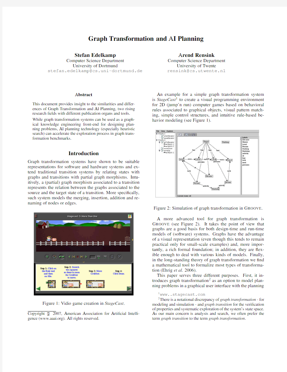
Figure1:Vidio game creation in StageCast. Copyright c 2007,American Association for Arti?cial Intelli-gence(https://www.wendangku.net/doc/9617680536.html,).All rights reserved.
An example for a simple graph transformation system is StageCast1to create a visual programming environment for2D(jump’n run)computer games based on behavioral rules associated to graphical objects,visual pattern match-ing,simple control structures,and intuitive rule-based be-havior modeling(see Figure
1).
Figure2:Simulation of graph transformation in G ROOVE.
A more advanced tool for graph transformation is G ROOVE(see Figure2).It takes the point of view that graphs are a good basis for both design-time and run-time models of(software)systems.Graphs have the advantage of a visual representation(even though this tends to remain practical only for small-scale examples)and,more impor-tantly,a rich formal foundation;in addition,they are?ex-ible enough to deal with various kinds of models.Finally, in the long-standing theory of graph transformation we?nd a mathematical tool to formalize most types of transforma-tion(Ehrig et al.2006).
This paper serves three different purposes.First,it in-troduces graph transformation2as an option to model plan-ning problems in a graphical user interface with the planning https://www.wendangku.net/doc/9617680536.html,
2There is a notational discrepancy of graph transformation-for modeling and simulation-and graph transition for the veri?cation of properties and systematic exploration of the system’s state space. As our main concern is analysis and search,we often prefer the term graph transition to the term graph transformation.
goal as a left-hand side for an error speci?cation in the graph transformation system.
Second,we show that for some graph transformation domains,AI action planning systems show better explo-ration ef?ciencies by using planner-speci?c but problem-independent state-to-goal heuristics,and discuss the ad-vances of graph transformation of effective handling of dy-namic environments with inherent symmetries.
Third,the paper provides basic information necessary to deal with the graph transformation benchmark that featured the International Competition on Knowledge Engineering for Planning&Scheduling,which included G ROOVE as one simulator environment for studying different plan models.
Graph Transition Systems
In order to get a mathematical?avor,what graph transfor-mation is about,the following set of de?nitions brie?y intro-duces the theory of graph transition function for the single-pushout approach based on partial graph morphisms using a left and right rule application pair3.
De?nition1A graph is a tuple G= V G,E G,src G,tgt G where V G is a set of nodes,E G is a set of edges,src G,tgt G: E G→V G are a source and target functions.
Graphs usually have a distinguished start state which we denote with s G0,or just s0if G is clear from the context.
De?nition2A path in a graph G is an alternating sequence of nodes and edges represented as u0e0→u1...such that for each i≥0we have u i∈V G,e i∈E G,src G(e i)=u i and tgt G(e i)=u i+1,or,shortly u i e i→u i+1.
An initial path is a path starting at s G0.Finite paths are required to end at states.The length of a?nite path p is de-noted by|p|.The concatenation of two paths p,q is denoted by pq,where we require p to be?nite and end at the initial state of q.
De?nition3A graph morphismψ:G1→G2is a pair of
mappingsψV:V G
1→V G
2
,ψE:E G
1
→E G
2
such that
we haveψV?src G
1=src G
2
?ψE,ψV?tgt G
1
=tgt G
2
?ψE.
A graph morphismψ:G1→G2is called injective if so are ψV andψE;identity if bothψV andψE are identities,and isomorphism if bothψE andψV are bijective.A graph G is a subgraph of graph G,if V G ?V G and E G ?E G,and the inclusions form a graph morphism.
A partial graph morphismψ:G1→G2is a pair G 1,ψm ,where G 1is a subgraph of G1,and whereψm: G 1→G2is a graph morphism.
The composition of(partial)graph morphisms results into another(partial)graph morphism.Now,we de?ne a notion of transition system.
3For the double-pushout approach each rule consists of a triple of left-hand side,invariant and a right-hand side.A rule speci?es that an occurrence of the left-hand side L in a larger graph G can be rewritten into the right hand side R preserving the interface K. For more information see(Corradini et al.2006).De?nition4A transition system is a graph M= S M,T M,in M,out M whose nodes and edges are respec-tively called states and transitions,with in M,out M repre-senting the source and target of an edge respectively. Finally,we are ready to de?ne graph transition systems, which are transition systems together with morphisms map-ping states into graphs and transitions into partial graph mor-phisms.
De?nition5A graph transition system is a pair M,g , where M is a transition system and g:M→U(G p)is a graph morphism from M to the graph underlying G p,the category of graphs with partial graph morphisms.There-fore g= g S,g T ,and the component on states g S maps each state s∈S M to a graph g S(s),while the component on transitions g T maps each transitions t∈T M to a partial graph morphism g T(t):g S(in M(t))?g S(out M(t)).
The G ROOVE Simulator
The G ROOVE project(Kastenberg&Rensink2006)aims at the usage of model checking techniques for verifying object-oriented systems,where the states of the system are modeled as graphs,instead of bit vectors as in most explicit state rep-resenting approaches.This approach creates new opportuni-ties to specify and verify systems in which the states mainly depend on a set of reference values instead of values of primitive types(with a?nite domain)only.Due to frequent (de)allocation of reference values,the states of such systems are highly dynamic,due to their variable size.Graphs pro-vide a natural way of representing the states of such systems and specifying interesting properties.The tool4follows the single-pushout approach as introduced above.
The G ROOVE simulator(Rensink2004)does a small part of the job of a model checker:it attempts to generate the full state space of a given graph grammar.This entails recur-sively computing and applying all enabled graph production rules at each state.Each newly generated state is compared to all known states up to isomorphism;matching states are merged(Rensink2003).No provisions are currently made for detecting or modeling in?nite state spaces.Alternatively, one may choose to simulate productions manually.The tool is designed for extensibility.The internal and visual repre-sentation of graphs are completely separated,and interfaces abstract from graph and morphism implementations.
The G ROOVE simulator is implemented in Java.The tool can handle arbitrary production rules,but can obviously only generate a?nite part of the corresponding graph transi-tion system.The simulator uses non-attributed,edge-labeled graphs without parallel edges.Node labels are actually la-bels of self-edges.The most performance critical parts of the simulator are:?nding rule matchings,and checking graph isomorphism.The?rst problem is,in general,NP-complete; the second is in NP but its precise time complexity classi?-cation is unknown(Wegener2003).
The modularity of G ROOVE also extends to the serial-ization and storage of graphs and graph grammars.Cur-rently the tool uses GXL(Winter,Kullbach,&Riediger https://www.wendangku.net/doc/9617680536.html,/projects/groove
2002),but in an ad hoc fashion:production rules are?rst encoded as graphs and then saved individually;thus,a gram-mar is stored as a set of?les.A sample GXL speci?cation is provided in the Appendix.Some performance?gures on G ROOVE were reported in(Rensink2004).
Modeling Planning Problems in G ROOVE We have seen that graph transformation systems enable users to encode domain models including states and tran-sition rules in form of graphs.This section gives insights and examples of applying graph transformation techniques for specifying and simulating action planning domains in a graphical interface.We further illustrate the impact of plan-ners in solving some graph transition problems faster than with current technology.For the sake of simplicity,we re-strict to propositional planning even if G ROOVE has been recently extended to deal with numeric attributes.
Action planning refers to a state space description in logic.
A number of atomic propositions describe what can be true or false in each state.By applying actions in a state,we arrive at another state where different atoms might be true or https://www.wendangku.net/doc/9617680536.html,ually,only some few atoms are affected by an action,and most of them remain the same.A concise rep-resentation the STRIPS formalism(Fikes&Nilsson1971), an acronym for an early planning system developed at Stan-ford University.STRIPS planning assumes a closed world. Everything that is not stated as being true is assumed to be false.Therefore,the denotation of the a state is shorthand for the value assignment to true of the propositions that are included in the state,and to false of the ones that are not.Ad-vances to STRIPS have let to the problem domain descrip-tion language PDDL(McDermott2000;Long&Fox2003; Hoffmann&Edelkamp2005).
Blocksworld
In Blocksworld a robot tries to reach a target state by actions that stack and unstack blocks,or put them on the table.In Fig.3we show a G ROOVE model the four operations stack, unstack,pickup,and putdown.Nodes represent objects types (in this case there is only one)and edges represent predicates that combine object types.Edges attached with new corre-spond to add effects,while edges labeled by del abbreviate delete effects.Delete edges together with persistent edges (none for Blocksworld)form the preconditions of the rule. Figure4illustrates the speci?cation of the initial state in G ROOVE.We?nd block B on top of block B and a singleton block A on the table.The robot arm is empty.Finally,Fig-ure5depicts the(entire)graph transition system that is gen-erated by continousely applying the4rules starting from the initial state,where rule application is established by match-ing the rule to the graph representing the current state. Logistics
An example for a more complex STRIPS domain is Logis-tics.The task is to transport packages within cities using trucks,and between cities airplanes.Locations within a city are connected and trucks can move between any two such locations.In each city there are one truck and one
airport.
stack
unstack
putdown pickup
Figure3:The graph transformation rules for
Blocksworld.
Figure4:The initial state for Blocksworld.
Fig.6shows the modeling of the actions as a graph trans-formation rule in G ROOVE.With Trucks,Airplane,Location and Packages four object types are used.Context edges like do not incur changes such as in for the drive action.
Running a Planner on G ROOVE Models
In this section we address the capability of modern planning in solving one of the problems that have been denoted as a challenge to graph transformation(Rensink2006).
The Girl’s Gossip Problem
There is a number of n girls,each of which has her own secret and one call action.On a call both participating girls divulge all the secrets they know.The question is,what is the minimal number of alls after which all girls know all secrets.The know optimum is2n?4calls.
The problem has been modeled as a graph transition sys-tem.In the following,we give an intuitive PDDL description for it utilizing conditional effects and bounded quanti?ca-tion.For the only action speci?cation we have
(:action call
:parameters(?g1?g2-girl)
:effect(and(forall(?s-secret)
(when(has-secret?g1?s)(has-secret?g2?s))) (forall(?s-secret)
(when(has-secret?g2?s)(has-secret?g1?s)))))
Figure 5:The state space generated from the initial state by the rule
set.
drive
?y
load-truck
unload-truck
load-airplane unload-airplane
Figure 6:The graph transformation rules for Logistics.The goal condition is that all girls know all secrets and corresponds to the requirement
(:goal (and
(forall (?g -girl)
(forall (?s -secret)(has-secret ?g ?s)))))
Table 1shows the result of running a planner in compari-son with two documented versions of G ROOVE to illustrate the exponential gain of heuristic search state space search 5.In the heuristic search planner FF (Hoffmann &Nebel 2001)we choose best-?rst instead of enforced hill-climbing,as the former delivers plans that are non-optimal.We have applied weighted A*,with an inadmissible heuristic weight factor of 2.Hence,there was no guarantee that the established
5
The experiments were run on a Windows Laptop with 512MB and 3GHz Pentium 4processor.
G ROOVE Plain G ROOVE Quant.FF girls states sec states sec states sec 53812.1.164,44811.1.1780,394240.1.182,309,76313,30860,9901,400.19--2,132,21087,302.111----635121----5,17039Table 1:Comparison of G ROOVE with the AI planner FF on the girl’s gossiping problem.
solution has a minimal number of steps.As we knew the minimal number of steps beforehand,we could,however,validate that the generated solutions of the planner were in-deed optimal.
The Dining Philosophers
In Dijkstra’s dining philosophers problem n philosophers sit around a table to have lunch.There are n plates,one for each philosopher,and n forks located to the left and to the right of each plate.Since two forks are required to eat the spaghetti on the plates,not all philosopher can eat at a time.Moreover,no communication except taking and releasing the forks takes place.The task is to devise a local strategy for each philosopher that lets all philosophers eventually eat.The simplest solution to access the left fork followed by the right one,has an obvious problem.If all philosopher wait for the second fork to be released there is no possible progress;a dead-end has occurred.
Studies in model checking (Edelkamp,Leue,&Lluch-Lafuente 2004)show that heuristic search for deadlocks scales well for this https://www.wendangku.net/doc/9617680536.html,ing an automated trans-lation from Promela inputs 6,a PDDL model for the din-ing philosopher problem was generated fully automatically.This benchmark has then be used in the 4th International Planning Competition (Hoffmann et al.2006).Here we pro-vide a simpli?ed PDDL model for the dining philosophers,equivalent to the one that is provided in G ROOVE .
(:action get-left
:parameters (?p1?p2-phil ?f -fork):precondition
(and (right ?p1?f)(left ?p2?f)(hungry ?p2)
(not (hold ?p1?f)))
:effect (and (hasLeft ?p2)(hold ?p2?f)
(not (hungry ?p2))))(:action get-right
:parameters (?p1?p2-phil ?f -fork):precondition
(and (right ?p1?f)(left ?p2?f)(hasLeft ?p1)
(not (hold ?p2?f)))
:effect (and (not (hasleft ?p1))(hold ?p1?f)
(eat ?p1)))
6
Promela is the input language of the model checker SPIN (Holzmann 2003)
(:action go-hungry
:parameters(?p-phil)
:precondition(and(think?p))
:effect(and(not(think?p))(hungry?p)))
(:action release-left
:parameters(?p-phil?f-fork)
:precondition(and(eat?p)(hold?p?f)
(left?p?f))
:effect(and(not(hold?p?f))(not(eat?p))
(hasright?p)))
(:action release-right
:parameters(?p-phil?f-fork)
:precondition(and(hold?p?f)(right?p?f)
(hasright?p))
:effect(and(think?p)(not(hold?p?f))
(not(hasright?p)))
Competition Usage
Graph transformation was one of the benchmark for the second International Knowledge Engineering Competition. Competitors and tools did not had to operate on the generic domain of graph transition systems,but to work on the indi-vidual graph transformation benchmarks instead.The dec-laration of the according graph transformation systems was be made available to the competitors.
This section is the manual of the graph transformation G ROOVE simulator as used in the competition.As with G ROOVE,its simulator wrapper is implemented in Java, while the server interface is written in c/c++.We brie?y describe the installation and invocation of the G ROOVE sim-ulator as a server application.
Running the Simulator
The simulator is invoked as follows:
GROOVE
The simulator then simulates the plan on the graph trans-formation problem and prints a report of the simulation to some?les starting with pre?x.The simulator executable is implemented as a wrapper in form of a bash script.
Most benchmarks are optimization problems minimizing the number of steps.The importance here is that there are more than one match to a rule such that a plan actually spans a tree of possible plan executions.So instead of the G ROOVE simulator that interactively allows to execute a sequence of matches,actually the G ROOVE transition system generator is invoked.A plan is reported to be valid if one of the execu-tion traces ends up in a?nal state.Moreover,all reachable states that can be generated given the generated plan are re-turned to the client.Example
For example,we take the list append problem(Rensink 2004)with the three rules,next,append and return. The example shows many features typical for the dynam-ics of object-oriented programs.Methods are modeled by nodes,with local variables as outgoing edges,including a this-labeled edge pointing to the object executing the method.Each method invocation results in a fresh node, with a caller edge to the invoking method.Upon return,the method node is deleted,while creating a return edge from its caller to a return value.It follows that the execution stack is represented by a chain of method nodes.List graph con-tain concurrently enabled method invocations;we expect the planner to tell us whether these invocations may interfere.A plan?le might look as follows
next next next append return
This simple plan(ordered list of transitions)syntax is the one ingested by the simulator.As such plan has many possi-ble outcomes all are reported.By applying the sequence in the example problem two possible states are generated and stored in the?les?les
Dif?culty Level
We have selected graph transformation benchmark domains of rising dif?culty.
?level1:Solitaire,Girls’Gossiping
?level2:List Manipulation,Circular Buffers
?level3:Balanced Search Trees
?level4:Virtual Machine
The description of the individual domains and the corre-sponding graph transformation systems were made available to the competitors.While Girls’Gossiping,List Manipula-tion,Circular Buffers existed before the competition,Soli-taire and Balanced Search Trees are new.The Virtual Ma-chine is the most complex graph transition model and has been described in(Kastenberg,Kleppe,&Rensink2006).
Conclusion and Discussion
This paper introduces to the interconnection between plan-ning and exploration in graph transformation systems.We used the G ROOVE simulator as a case study,and showed that some traditional STRIPS planning benchmarks can be speci?ed intuitively7.The interface for de?ning graph trans-formation system uses XML8.
The paper also delivers?rst data for possible synergies opposite direction,i.e.,how planner can accelerate the ex-ploration process for graph transformation systems for a spe-ci?c target graph.We have seen a PDDL description for a 7Besides Blocksworld and Logistics we also successfully mod-eled the Grid and Gripper domain in G ROOVE.
8An overview on the status quo on the language development of GXL and GTXL can be found at http://tfs.cs.tu-berlin.de/projekte/gxl-gtxl.html.
problem that has been identi?ed as a challenge and shown that planners can be superior to state-of-the-art technologies. In(Edelkamp,Jabbar,&Lluch-Lafuente2005)the mod-eling of graph transition systems in PDDL and the applica-tion of heuristic search planning for their analysis are dis-cussed for the?rst time applying different heuristics in a case study on the arrow distributed directory protocol(Dem-mer&Herlihy1998).
Nonetheless the expressiveness of planners and model checkers based on graph transformation are different.On the one hand modern PDDL planners cover numerical attributes for optimizing objective functions,they allow to attach du-ration to rules for?nding schedules of when to apply which rules to minimize the makespan.Recent additions to PDDL also cover additional soft constraints to be imposed on the set of feasible plans.
On the other hand,graph transformation systems like G ROOVE feature untyped domain objects to allow the gen-eration of a symmetry reduced state space.Two isomorphic graphs are represented only ones.Assigning names to ob-jects,as done in planning actually destroys these symme-tries.Moreover,G ROOVE covers dynamic aspects such as objects and predicate creation that are not dealt with yet in the PDDL language.
We chose G ROOVE as it is self-contained,platform in-dependent,relatively stable,available to public domain and because the simulator is attached to a state space gener-ator.Another simulator for graph transformation systems is AGG9.AGG features many different options such as ef-?cient matching,consistency checking,and a critical pair analysis.An alternative for the veri?cation of systems with graph transformation is AUGUR(K¨o nig&Kozioura 2005).Recent developments in AUGUR unfold and approx-imate the graph transformation system in form of a Petri-Net(K¨o nig&Kozioura2006).
Recent work by(Zaks2007)shows that?nding counter-example in Petri-Net approximations within a graph trans-formation re?nement loop is seemingly faster when export-ing the domain to PDDL and use a from-shelf action planner planner.In his work,the author compares the planner Met-ricFF with the Petri Net reachability analyzer BWRA.The following table shows selected run-time results(in seconds).
Problem BWRA MetricFF Error
red-black9471yes
red-black9481yes
?rewall271yes
?rewall23381yes
?rewall261yes
server21–no
server26–no
server25451yes
For International Knowledge Engineering Competition we summarize the important contributions of our work, which makes graph transformation an appropriate candidate for a benchmark domain.
9See http://tfs.cs.tu-berlin.de/agg ?Graph transformation systems provide an?exible,intu-itive input speci?cation for systems of change with a sound mathematical basis.The geometric layout of the graphs associates semantics to the syntactical structures. Vied that way,simulators like G ROOVE can be seen as a knowledge engineering framework for specifying plan-ning problems.With this respect,we establish a tight connection to the KE tool ItSimple(Vaquero et al.2006; Vaquero,Tonidande,&Silva2007).
G ROOVE has been recently extended to certain form of arithmetics on the attributes(Kastenberg2005),so that more expressive numerical plan models can be simulated.?Graph transformation system bridge the gap between speci?cation and software veri?cation as they allow to validate certain types of UML designs and software mod-els.With the incorporation of heuristic/local search plan-ners,bug?nding as proposed in the directed model check-ing paradigm can be accelerated.A planner input com-pilation includes tool-inherent guidance to the search for free,while heuristics for graph transformation systems have not yet been implemented(Edelkamp,Jabbar,& Lluch-Lafuente2006)
?The main objective of this article is to provide a challeng-ing domain for the design of plan models.The number of graph transformation benchmark problems is continu-ously rising10even though no forum yet exists11
To steer G ROOVE remotely,a?le or protocol-base sim-ulation has been provided.This has imposed only a minor extension to the public release of G ROOVE.
Acknowledgments
The?rst author thanks DFG for support in the projects Di-rected Model Checking and Heuristic Search,Reiko Heckel for the link to StageCast,and Barbara K¨o nig for joint super-vision of the master thesis of Maxim Zaks.
References
Corradini,A.;Ehrig,H.;Montanari,U.;Ribeiro,L.;and Rozenberg,G.,eds.2006.Graph Transformation.Pro-ceedings of the3rd International Conference.Springer, Lecture Notes in Computer Science,V olume4178. Demmer,M.J.,and Herlihy,M.1998.The arrow dis-tributed directory protocol.In In International Symposium on Distributed Computing(DISC),119–133. Edelkamp,S.;Jabbar,S.;and Lluch-Lafuente,A.2005. Action planning for graph transition systems.In ICAPS-Workshop on Veri?cation and Validation of Model-Based Planning and Scheduling Systems(VVPS),58–66.
10In the?rst graph transformation contest on AGTIVE-07Ludo, UML-to-CSP,Sierpinsky triangles were posed.
11Examples in GXL language(single push-out)like list manipulation and buffer manipulation come with the G ROOVE distribution,while(double pushout)ex-amples like mutual exclusion,dining philosophers and red-black trees,de?ned in GTXL can be obtained on http://www.ti.inf.uni-due.de/research/
augur1/examples/index.shtml
Edelkamp,S.;Jabbar,S.;and Lluch-Lafuente,A.2006. Heuristic search for the analysis of graph transition sys-tems.In International Conference on Graph Transforma-tion(ICGT),414–429.
Edelkamp,S.;Leue,S.;and Lluch-Lafuente,A.2004.Di-rected explicit-state model checking in the validation of communication protocols.International Journal on Soft-ware Tools for Technology5(2-3):247–267.
Ehrig,H.;Ehrig,K.;Prange,U.;and Taentzer,G. 2006.Fundamentals of Algebraic Graph Transformation. Springer.
Fikes,R.,and Nilsson,N.1971.STRIPS:A new approach to the application of theorem proving to problem solving. Arti?cial Intelligence2:189–208.
Hoffmann,J.,and Edelkamp,S.2005.The deterministic part of IPC-4:An overview.Journal of Arti?cial Intelli-gence Research24:519–579.
Hoffmann,J.,and Nebel,B.2001.Fast plan generation through heuristic search.Journal of Arti?cial Intelligence Research14:253–302.
Hoffmann,J.;Edelkamp,S.;Thiebaux,S.;Englert,R.;Li-porace,F.;and Tr¨u g,S.2006.Engineering realistic bench-marks for planning:the domains used in the deterministic part of IPC-4.Journal of Arti?cial Intelligence Research 453–542.
Holzmann,G.J.2003.The SPIN Model Checker.Addison-Wesley.
Kastenberg,H.,and Rensink,A.2006.Model checking dynamic states in GROOVE.In Model Checking Software (SPIN),299–305.
Kastenberg,H.;Kleppe,A.;and Rensink,A.2006.De?n-ing object-oriented execution semantics using graph trans-formations.In Formal Methods for Open Object-Based Distributed System(FMOODS),186–201. Kastenberg,H.2005.Towards attributed graphs in Groove. 154(2):47–54.
K¨o nig,B.,and Kozioura,V.2005.Augur—a tool for the analysis of graph transformation systems.EATCS Bulletin 87:125–137.Appeared in The Formal Speci?cation Col-umn.
K¨o nig,B.,and Kozioura,V.2006.Counterexample-guided abstraction re?nement for the analysis of graph transforma-tion systems.In TACAS,197–211.
Long,D.,and Fox,M.2003.The3rd international plan-ning competition:Overview and results.JAIR20.Special issue on the3rd International Planning Competition. McDermott,D.2000.The1998AI Planning Competition. AI Magazine21(2).
Rensink,A.2003.Towards model checking graph gram-mars.Technical Report DSSETR20032,Proceedings of the 3rd Workshop on Automated Veri?cation of Critical Sys-tems.University of Southampton.
Rensink,A.2004.The Groove simulator:A tool for state space generation.In Applications of Graph Transforma-tions with Industrial Relevance(AGTIVE),479–485.
Rensink,A.2006.Nested quanti?cation in graph transfor-mation rules.In International Conference on Graph Trans-formation(ICGT),1–13.
Vaquero,T.S.;Tonidande,F.;de Barrow,L.N.;and Silva, J.R.2006.On the use of UML.P for modeling a real appli-cation as a planning problem.In International Conference on Automated planning and Scheduling(ICAPS),434–437. Vaquero,T.S.;Tonidande,F.;and Silva,J.R.2007.it-simple2.0:An integrated tool for designing planning do-mains.In International Conference on Automated planning and Scheduling(ICAPS).To appear.
Wegener,I.2003.Komplexit¨a tstheorie.Springer. Winter,A.;Kullbach,B.;and Riediger,V.2002.An overview of the GXL graph exchange language.In Soft-ware Visualization,324–336.Springer,LNCS.
Zaks,M.2007.Ef?cient algorithms for the analysis of graph transformation systems.Master’s thesis.
Appendix
GXL of the stack rule of the Blocksworld domain.
edgemode="directed">
Windows系统自带画图工具教程87586
1.如何使用画图工具 想在电脑上画画吗?很简单,Windows 已经给你设计了一个简洁好用的画图工具,它在开始菜单的程序项里的附件中,名字就叫做“画图”。 启动它后,屏幕右边的这一大块白色就是你的画布了。左边是工具箱,下面是颜色板。 现在的画布已经超过了屏幕的可显示范围,如果你觉得它太大了,那么可以用鼠标拖曳角落的小方块,就可以改变大小了。 首先在工具箱中选中铅笔,然后在画布上拖曳鼠标,就可以画出线条了,还可以在颜色板上选择其它颜色画图,鼠标左键选择的是前景色,右键选择的是背景色,在画图的时候,左键拖曳画出的就是前景色,右键画的是背景色。
选择刷子工具,它不像铅笔只有一种粗细,而是可以选择笔尖的大小和形状,在这里单击任意一种笔尖,画出的线条就和原来不一样了。 图画错了就需要修改,这时可以使用橡皮工具。橡皮工具选定后,可以用左键或右键进行擦除,这两种擦除方法适用于不同的情况。左键擦除是把画面上的图像擦除,并用背景色填充经过的区域。试验一下就知道了,我们先用蓝色画上一些线条,再用红色画一些,然后选择橡皮,让前景色是黑色,背景色是白色,然后在线条上用左键拖曳,可以看见经过的区域变成了白色。现在把背景色变成绿色,再用左键擦除,可以看到擦过的区域变成绿色了。 现在我们看看右键擦除:将前景色变成蓝色,背景色还是绿色,在画面的蓝色线条和红色线条上用鼠标右键拖曳,可以看见蓝色的线条被替换成了绿色,而红色线条没有变化。这表示,右键擦除可以只擦除指定的颜色--就是所选定的前景色,而对其它的颜色没有影响。这就是橡皮的分色擦除功能。 再来看看其它画图工具。 是“用颜料填充”,就是把一个封闭区域内都填上颜色。 是喷枪,它画出的是一些烟雾状的细点,可以用来画云或烟等。 是文字工具,在画面上拖曳出写字的范围,就可以输入文字了,而且还可以选择字体和字号。 是直线工具,用鼠标拖曳可以画出直线。
LAMMPS手册-中文版讲解之欧阳家百创编
LAMMPS手册-中文解析 一、 欧阳家百(2021.03.07) 二、简介 本部分大至介绍了LAMMPS的一些功能和缺陷。 1.什么是LAMMPS? LAMMPS是一个经典的分子动力学代码,他可以模拟液体中的粒子,固体和汽体的系综。他可以采用不同的力场和边界条件来模拟全原子,聚合物,生物,金属,粒状和粗料化体系。LAMMPS可以计算的体系小至几个粒子,大到上百万甚至是上亿个粒子。 LAMMPS可以在单个处理器的台式机和笔记本本上运行且有较高的计算效率,但是它是专门为并行计算机设计的。他可以在任何一个按装了C++编译器和MPI的平台上运算,这其中当然包括分布式和共享式并行机和Beowulf型的集群机。 LAMMPS是一可以修改和扩展的计算程序,比如,可以加上一些新的力场,原子模型,边界条件和诊断功能等。 通常意义上来讲,LAMMPS是根据不同的边界条件和初始条件对通过短程和长程力相互作用的分子,原子和宏观粒子集合对它们的牛顿运动方程进行积分。高效率计算的LAMMPS通过采用相邻清单来跟踪他们邻近的粒子。这些清单是根据粒子间的短程互拆力的大小进行优化过的,目的是防止局部粒子密度过高。在
并行机上,LAMMPS采用的是空间分解技术来分配模拟的区域,把整个模拟空间分成较小的三维小空间,其中每一个小空间可以分配在一个处理器上。各个处理器之间相互通信并且存储每一个小空间边界上的”ghost”原子的信息。LAMMPS(并行情况)在模拟3维矩行盒子并且具有近均一密度的体系时效率最高。 2.LAMMPS的功能 总体功能: 可以串行和并行计算 分布式MPI策略 模拟空间的分解并行机制 开源 高移植性C++语言编写 MPI和单处理器串行FFT的可选性(自定义) 可以方便的为之扩展上新特征和功能 只需一个输入脚本就可运行 有定义和使用变量和方程完备语法规则 在运行过程中循环的控制都有严格的规则 只要一个输入脚本试就可以同时实现一个或多个模拟任务 粒子和模拟的类型: (atom style命令) 原子 粗粒化粒子 全原子聚合物,有机分子,蛋白质,DNA
细节决定成败——认识“画图”软件教学案例
细节决定成败 ——认识“画图”软件教学案例 【事件背景】 2014年9月29日按照学校教学安排,把精心准备的《认识“画图”软件》一课在学科组内做了认真的课堂展示。这节课是小学三年级的课,前节课学生初步认识了纸牌游戏软件,对在Windows中打开软件、认识窗口有了初步的了解。但是学生初学画图,鼠标拖动操作还不熟练,在技巧上还有待于逐步尝试掌握。根据学生原有的水平我提出了一个设计思路,即“作品欣赏,激发兴趣,互相讨论,任务驱动,指导点评”。 课堂中重难点的处理我主要是采用任务驱动教学法,设置了三个学习任务,分别以不同形式完成。对于第一个任务:启动“画图”软件,让学生自学教材P31,完成“画图”软件的启动。是为培养学生的自主学习能力,多数学生都能顺利启动后,找两个同学示范启动,锻炼了学生的动手操作和语言表达能力。第二个任务:认识“画图”软件的窗口组成我主要是用事先录制好的微课展示让学生记住。学生对这种形式感到很新奇,自然很快就记住了。第三个任务是这节课的重点也是难点:尝试用画图工具简单作画。 【事件描述】 根据教学设计,我全身心的投入到本节课的教学实践之中,课堂伊始效果良好,学生不仅对学习内容表现出了极大的兴趣,而且行为表现也很规范,学习状态认真。所以很顺畅的完成了第一个学习任务,紧接着便进入第二个环节的学习,即认识画图软件的窗口。为了很好的完成这一重要的学习任务,我对教学设计几经修改,最后决定采用‘微课’的形式,我便精心制作课件,录音合成,以图示加拟人风格的自述形式进行软件的自我介绍。当初我想这样做一定会收到事半功倍的效果,期待着在课堂上那称心一幕的出现。事实又是怎样的呢?
最新pymol作图的一个实例
Pymol作图的实例 这是一个只是用鼠标操作的初步教程 Pdb文件3ODU.pdb 打开文件 pymol右侧 All指所有的对象,2ODU指刚才打开的文件,(sele)是选择的对象 按钮A:代表对这个对象的各种action, S:显示这个对象的某种样式, H:隐藏某种样式, L:显示某种label, C:显示的颜色 下面是操作过程: 点击all中的H,选择everything,隐藏所有 点击3ODU中的S,选择cartoon,以cartoon形式显示蛋白质 点击3ODU中的C,选择by ss,以二级结构分配颜色,选择 点击右下角的S,窗口上面出现蛋白质氨基酸序列,找到1164位ITD,是配体 点击选择ITD ,此时sele中就包含ITD这个残基,点击(sele)行的A,选 择rename selection,窗口中出现,更改sele 为IDT,点击(IDT)行的S选择sticks,点击C,选择by element,选择,,调 整窗口使此分子清楚显示。 寻找IDT与蛋白质相互作用的氢键: IDT行点击A 选择find,选择polar contacts,再根据需要选择,这里选择to other atoms in object ,分子显示窗口中出现几个黄色的虚线,IDT行下面出现了新的一行,这就是氢键的对象,点击这一行的C,选择 red red,把氢键显示为红色。 接着再显示跟IDT形成氢键的残基 点击3ODU行的S,选择lines,显示出所有残基的侧链,使用鼠标转动蛋白质寻找与IDT 以红色虚线相连的残基,分别点击选择这些残基。注意此时selecting要是
residures。选择的时候要细心。取消选择可以再次点击已选择的残基。使用上述的方法把选择的残基(sele)改名为s1。点击S1行的S选择sticks,C选择by elements,点击L选择residures显示出残基名称.在这个例子中发现其中有一个N含有3个氢键有两个可以找到与其连接的氨基酸残基,另一个找不到,这是因为这个氢键可能是与水分子形成的,水分子在pdb文件中只用一个O表示,sticks显示方式没有显示出来水分子,点击all行S选择nonbonded,此时就看到一个水与N形成氢键 ,点击分子空白处,然后点击选择这个水分子,更改它的名字为w。在all 行点击H,选择lines,在选择nonbonded,把这些显示方式去掉只留下cartoon。点击w行s 选择nb-spheres. 到目前为止已经差不多了 下面是一些细节的调整 残基名称位置的调整:点击右下角是3-button viewing 转变为3-button viewing editing,这样就可以编辑修改 pdb文件了,咱们修改的是label的位置。按住ctrl键点击窗口中的残基名称label,鼠标拖拽到适合的部位,是显示更清晰。 然后调整视角方向直到显示满意为止,这时就可以保存图片了,file>>save image as>>png
最全的几何画板实例教程
上篇用几何画板做数理实验 图1-0.1 我们主要认识一下工具箱和状态栏,其它的功能在今后的学习过程中将学会使用。 案例一四人分饼 有一块厚度均匀的三角形薄饼,现在要把它平 均分给四个人,应该如何分? 图1-1.1 思路:这个问题在数学上就是如何把一个三角形分成面积相等的四部分。 方案一:画三角形的三条中位线,分三角形所成的四部 分面积相等,(其实四个三角形全等)。如图1-1.2。 图1-1.2
方案二:四等分三角形的任意一边,由等底等高的三角 形面积相等,可以得出四部分面积相等,如图1-1.3。 图1-1.3 用几何画板验证: 第一步:打开几何画板程序,这时出现一个新绘图文件。 说明:如果几何画板程序已经打开,只要由菜单“文件” “新绘图”,也可以新建一个绘图文件。第二步:(1)在工具箱中选取“画线段”工具; (2)在工作区中按住鼠标左键拖动,画出一条线段。如图 1-1.4。 注意:在几何画板中,点用一个空心的圈表示。 图1-1.4 第三步:(1)选取“文本”工具;(2)在画好的点上单击左 键,可以标出两点的标签,如图1-1.5: 注意:如果再点一次,又可以隐藏标签,如果想改标签 为其它字母,可以这样做: 用“文本”工具双击显示的标签,在弹出的对话框中进 行修改,(本例中我们不做修改)。如图1-1.6 图1-1.6 在后面的操作中,请观察图形,根据需要标出点或线的 标签,不再一一说明 B 图1-1.5 第四步:(1)再次选取“画线段”工具,移动鼠标与点A 重合,按左键拖动画出线段AC;(2)画线段BC,标出标 签C,如图1-1.7。 注意:在熟悉后,可以先画好首尾相接的三条线段后再 标上标签更方便。 B 图1-1.7
画图工具教程
画图工具阶段教学指引如何使用画图工具 画图工具妙用文字工具 画图工具妙用圆形工具 画图工具妙用曲线工具 如何让画图工具存JPG格式 Win98 画图工具持JPG图片一法 Win98 画图工具持JPG图片二法 画图工具应用之屏幕拷贝 画图工具应用之双色汉字 画图工具应用之放大修改 画图工具应用之工具与颜色配置 画图工具应用之灵活编辑 画图工具操作技巧 画图工具应用技巧 画图工具另类技巧检测LCD的暗点
如何使用画图工具 想在电脑上画画吗?很简单,Windows 已经给你设计了一个简洁好用的画图工具,它在开始菜单的程序项里的附件中,名字就叫做“画图”。 启动它后,屏幕右边的这一大块白色就是你的画布了。左边是工具箱,下面是颜色板。 现在的画布已经超过了屏幕的可显示范围,如果你觉得它太大了,那么可以用鼠标拖曳角落的小方块,就可以改变大小了。 首先在工具箱中选中铅笔,然后在画布上拖曳鼠标,就可以画出线条了,还可以在颜色板上选择其它颜色画图,鼠标左键选择的是前景色,右键选择的是背景色,在画图的时候,左键拖曳画出的就是前景色,右键画的是背景色。
选择刷子工具,它不像铅笔只有一种粗细,而是可以选择笔尖的大小和形状,在这里单击任意一种笔尖,画出的线条就和原来不一样了。 图画错了就需要修改,这时可以使用橡皮工具。橡皮工具选定后,可以用左键或右键进行擦除,这两种擦除方法适用于不同的情况。左键擦除是把画面上的图像擦除,并用背景色填充经过的区域。试验一下就知道了,我们先用蓝色画上一些线条,再用红色画一些,然后选择橡皮,让前景色是黑色,背景色是白色,然后在线条上用左键拖曳,可以看见经过的区域变成了白色。现在把背景色变成绿色,再用左键擦除,可以看到擦过的区域变成绿色了。 现在我们看看右键擦除:将前景色变成蓝色,背景色还是绿色,在画面的蓝色线条和红色线条上用鼠标右键拖曳,可以看见蓝色的线条被替换成了绿色,而红色线条没有变化。这表示,右键擦除可以只擦除指定的颜色--就是所选定的前景色,而对其它的颜色没有影响。这就是橡皮的分色擦除功能。 再来看看其它画图工具。 是“用颜料填充”,就是把一个封闭区域内都填上颜色。 是喷枪,它画出的是一些烟雾状的细点,可以用来画云或烟等。 是文字工具,在画面上拖曳出写字的范围,就可以输入文字了,而且还可以选择字体和字号。 是直线工具,用鼠标拖曳可以画出直线。 是曲线工具,它的用法是先拖曳画出一条线段,然后再在线段上拖曳,可以把线段上从拖曳的起点向一个方向弯曲,然后再拖曳另一处,可以反向弯曲,两次弯曲后曲线就确定了。 是矩形工具,是多边形工具,是椭圆工具,是圆角矩形,多边形工具的用法是先拖曳一条线段,然后就可以在画面任意处单击,画笔会自动将单击点连接
50款医学软件
一、PPT模板与软件: 1、ScienceSlides: ScienceSlides就是一种PPT插件,可方便的画出各种细胞器化学结构,用来论文画图确实很好用。特别就是用这个与AI(illustrator)结合,画的图可以媲美老外的CNS哦。 2、科研医学美图PPT模板 3、200+套绝美PPT模板 二、代谢与信号分析软件: 1、CellNetAnalyzer: CellNetAnalyzer,就是一种细胞网络分析工具,前身就是FluxAnalyzer,就是基于MatLab的代谢网络与信号传导网络分析模块,。这就是一个典型的代谢流分析工具,可以进行代谢流的计算、预测、目标函数的优化,端途径分析、元素模式分析,以及代谢流之间的对比等。可以基本满足研究一个中型代谢网络的结构尤其就是计算流分配的要求,大部分论文中的代谢网络分析都就是或明或暗的用这个分析的。
2、信号通路图汇总 3、药理学思维导图 三、二维、三维构图软件: 1、DeepViewer _4、10_PC DeepViewer ,曾经也叫做Swiss-PdbViewer,就是一个可以同时分析几个蛋白的应用程序。为了结构比对并且比较活性位点或者任何别的相关部分,蛋白质被分成几个层次。氨基酸突变,氢键,原子间的角与距离在直观的图示与菜单界面上很容易获得。 2、pymol-0_99rc6-bin-win32 PyMOL就是一个开放源码,由使用者赞助的分子三维结构显示软件。PyMOL适用于创作高品质的小分子或就是生物大分子(特别就是蛋白质)的三维结构图像。PyMOL的源代码目前仍可以免费下载,供使用者编译。对于Linux、Unix以及Mac OS X等操作系统,非付费用户可以通过自行编译源代码来获得PyMOL执行程式;而对于Windows的使用者,如果不安装第三方软件,则无法编译源代码。 四、分子生物学软件
pymol作图的一个实例
Pymol作图的实例 这就是一个只就是用鼠标操作的初步教程 Pdb文件3ODU、pdb 打开文件 pymol右侧 All指所有的对象,2ODU指刚才打开的文件,(sele)就是选择的对象 按钮A:代表对这个对象的各种action, S:显示这个对象的某种样式, H:隐藏某种样式, L:显示某种label, C:显示的颜色 下面就是操作过程: 点击all中的H,选择everything,隐藏所有 点击3ODU中的S,选择cartoon,以cartoon形式显示蛋白质 点击3ODU中的C,选择by ss,以二级结构分配颜色,选择 点击右下角的S,窗口上面出现蛋白质氨基酸序列,找到1164位ITD,就是配体 点击选择ITD ,此时sele中就包含ITD这个残基,点击(sele)行的A,选择rename selection,窗口中出现,更改sele为IDT,点击 (IDT)行的S选择sticks,点击C,选择by element,选择,,调整窗口使此分子清楚显示。 寻找IDT与蛋白质相互作用的氢键: IDT行点击A 选择find,选择polar contacts,再根据需要选择,这里选择to other atoms in object , 分子显示窗口中出现几个黄色的虚线,IDT行下面出现了新的一行 ,这就就是氢键的对象,点击这一行的C,选择red red,把氢键显示为红色。 接着再显示跟IDT形成氢键的残基 点击3ODU行的S,选择lines,显示出所有残基的侧链,使用鼠标转动蛋白质寻找与IDT以红色虚线相连的残基,分别点击选择这些残基。注意此时selecting要就是 residures。选择的时候要细心。取消选择可以再次点击已选择
认识画图软件教案
《认识画图软件》教学设计 任教教师:苗丽娟 所在学校:复兴小学
《认识画图软件》教学设计 教学目标: 1、能熟练启动并退出画图软件; 2、认识画图软件的窗口并了解各种绘画工具的使用; 3、能绘制简单的图形。 重点难点: 了解各种绘画工具的使用。 教学时间:一课时 课前准备: 课件 教学过程: 一、导入 1、今天的天气真好,阳光明媚,老师和大家一起来欣赏一些作品(出示课件) 师:这些画漂不漂亮,它们不仅漂亮而且还很神奇。因为不是用笔和纸画出来的,而是用电脑上的画图软件画出来的。同学们想不想成为一名电脑绘画小高手。那就和老师一起来学习这一课:认识画图软件(课件出示) 二、新授 1、启动画图软件: 课件出示启动画图软件的方法,请同学们根据课件演示操作。 2、认识画图软件窗口: 课件出示画图软件窗口。 3、认识工具箱 (1)师问:工具箱中有多少个按钮? 师:告诉大家一个方法,当我们把鼠标指针放到某个工具上时就会在它的旁边出现它的名字,而且下面任务栏中会出现对这个工具使用方法的介绍。 现在就请大家发挥你的小组合作能力,自主的探究一下这些工具: (2)课件出示:合作探究:工具箱中的各种工具有些什么作用?怎样使用?
(3)师说明活动要求:两人为一个小组进行合作,解决上述问题。 (4)学生操作。师和学生单独交流,了解学生学习情况,收集学生问题。(5)师问:谁愿意说说你对哪个工具最了解?它的名称是什么?怎样使用?(学生边说边演示,鼓励台下学生向台上演示的学生提出不懂的问题并寻求解决方法) 4、认识调色板: 课件出示选色框图:上面框中的颜色称为前景色,下面框中的颜色称为背景色 我们已经简单的认识了一些工具,现在我们画一个简单的图形并给它涂上颜色。 生画完后,师:在刚才的上色过程中为什么只有前景色会变化?背景色怎样改变?大家尝试一下。 师总结:单击左键拾取前景色,单击右键拾取背景色。 课件出示儿歌: 调色板儿真方便,多种颜色我来选。 单击左键前景色,单击右键背景色。 前景背景不一样,两键单击记心间。 三、退出画图软件 师:当图软件用完之后,怎样退出呢?聪明的你们能不能从课本上找到答案?有几种方法? 第一种: 单击“文件(F)”菜单中的“退出(X)”命令,可以退出“画图”程序。 第二种:按一下右上角的× 师:如果还没有保存画好或修改过的图形,则在退出“画图”程序时,屏幕上会出现“画图”对话框,这时,如果单击“是(Y)”按钮,则保存图形后再退出;如果单击“否(N)”按钮,则不保存图形就退出;如果单击“取消”按钮,则不退出“画图”程序。 四、赛一赛
pymol作图的一个实例演示教学
p y m o l作图的一个实 例
Pymol作图的实例 这是一个只是用鼠标操作的初步教程 Pdb文件3ODU.pdb 打开文件 pymol右侧 All指所有的对象,2ODU指刚才打开的文件,(sele)是选择的对象 按钮A:代表对这个对象的各种action, S:显示这个对象的某种样式, H:隐藏某种样式, L:显示某种label, C:显示的颜色 下面是操作过程: 点击all中的H,选择everything,隐藏所有 点击3ODU中的S,选择cartoon,以cartoon形式显示蛋白质 点击3ODU中的C,选择by ss,以二级结构分配颜色,选择 点击右下角的S,窗口上面出现蛋白质氨基酸序列,找到1164位ITD,是配体点击选择ITD ,此时sele中就包含ITD这个残基,点击(sele)行的A,选择rename selection,窗口中出现
,更改sele为IDT,点击(IDT)行的S选择sticks,点击C,选择by element,选择,,调整窗口使此分子清楚显示。 寻找IDT与蛋白质相互作用的氢键: IDT行点击A 选择find,选择polar contacts,再根据需要选择,这里选择to other atoms in object ,分子显示窗口中出现几个黄色的虚线 ,IDT行下面出现了新的一行 ,这就是氢键的对象,点击这一行的C,选择red red,把氢键显示为红色。 接着再显示跟IDT形成氢键的残基 点击3ODU行的S,选择lines,显示出所有残基的侧链,使用鼠标转动蛋白质寻找与IDT以红色虚线相连的残基,分别点击选择这些残基。注意此时selecting要是residures。选择的时候要细心。取消选择可以再次点击已选择的残基。使用上述的方法把选择的残基(sele)改名为s1。点击S1行的S选择sticks,C选择by elements,点击L选择residures显示出残基名称.在这个例子中发现其中有一个N含有3个氢键有两个可以找到与其连接的氨基酸残基,另一个找不到,这是因为这个氢键可能是与水分子形成的,水分子在pdb文件中只用一个O表示,sticks显示方式没有显示出来水分子,点击all行S选择nonbonded,此时就看到一个水与N形成氢键
使用画图工具
如何使用画图工具 想在电脑上画画吗?很简单,Windows 已经给你设计了一个简洁好用的画图工具,它在开始菜单的程序项里的附件中,名字就叫做 “画图”。 启动它后,屏幕右边的这一大块白色就是你的画布了。左边是 工具箱,下面是颜色板。 现在的画布已经超过了屏幕的可显示范围,如果你觉得它太大了,那么可以用鼠标拖曳角落的小方块,就可以改变大小了。 首先在工具箱中选中铅笔,然后在画布上拖曳鼠标,就可以画出线条了,还可以在颜色板上选择其它颜色画图,鼠标左键选择的是
前景色,右键选择的是背景色,在画图的时候,左键拖曳画出的就是前 景色,右键画的是背景色。 选择刷子工具,它不像铅笔只有一种粗细,而是可以选择笔尖的大小和形状,在这里单击任意一种笔尖,画出的线条就和原来不一 样了。 图画错了就需要修改,这时可以使用橡皮工具。橡皮工具选定后,可以用左键或右键进行擦除,这两种擦除方法适用于不同的情况。左键擦除是把画面上的图像擦除,并用背景色填充经过的区域。试验一下就知道了,我们先用蓝色画上一些线条,再用红色画一些,然后选择橡皮,让前景色是黑色,背景色是白色,然后在线条上用左键拖曳,可以看见经过的区域变成了白色。现在把背景色变成绿色,再用左键擦除,可以看到擦过的区域变成绿色了。 现在我们看看右键擦除:将前景色变成蓝色,背景色还是绿色,在画面的蓝色线条和红色线条上用鼠标右键拖曳,可以看见蓝色的线条被替换成了绿色,而红色线条没有变化。这表示,右键擦除可以只擦除指定的颜色--就是所选定的前景色,而对其它的颜色没有影响。 这就是橡皮的分色擦除功能。 再来看看其它画图工具。 是“用颜料填充”,就是把一个封闭区域内都填上颜色。 是喷枪,它画出的是一些烟雾状的细点,可以用来画云或烟 等。
CAD绘图教程及案例_很实用
CAD 绘制三维实体基础 AutoCAD除具有强大的二维绘图功能外,还具备基本的三维造型能力。若物体并无复杂的外表曲面及多变的空间结构关系,则使用AutoCAD可以很方便地建立物体的三维模型。本章我们将介绍AutoCAD 三维绘图的基本知识。 11.1 三维几何模型分类 在AutoCAD中,用户可以创建3种类型的三维模型:线框模型、表面模型及实体模型。这3种模型在计算机上的显示方式是相同的,即以线架结构显示出来,但用户可用特定命令使表面模型及实体模型的真实性表现出来。 11.1.1线框模型(Wireframe Model) 线框模型是一种轮廓模型,它是用线(3D空间的直线及曲线)表达三维立体,不包含面及体的信息。不能使该模型消隐或着色。又由于其不含有体的数据,用户也不能得到对象的质量、重心、体积、惯性矩等物理特性,不能进行布尔运算。图11-1显示了立体的线框模型,在消隐模式下也看到后面的线。但线框模型结构简单,易于绘制。 11.1.2 表面模型(Surface Model) 表面模型是用物体的表面表示物体。表面模型具有面及三维立体边界信息。表面不透明,能遮挡光线,因而表面模型可以被渲染及消隐。对于计算机辅助加工,用户还可以根据零件的表面模型形成完整的加工信息。但是不能进行布尔运算。如图11-2所示是两个表面模型的消隐效果,前面的薄片圆筒遮住了后面长方体的一部分。 11.1.3 实体模型 实体模型具有线、表面、体的全部信息。对于此类模型,可以区分对象的内部及外部,可以对它进行打孔、切槽和添加材料等布尔运算,对实体装配进行干涉检查,分析模型的质量特性,如质心、体积和惯性矩。对于计算机辅助加工,用户还可利用实体模型的数据生成数控加工代码,进行数控刀具轨迹仿真加工等。如图11-3所示是实体模型。 图11-1 线框模型 图11-2 表面模型 1、三维模型的分类及三维坐标系; 2、三维图形的观察方法; 3、创建基本三维实体; 4、由二维对象生成三维实体; 5、编辑实体、实体的面和边;
《画图软件画图忙》教学设计
《画图软件画图忙》教学设计 [教学目标] (1)学习启动与退出“画图”程序。 (2)了解“画图”窗口的组成,特别是画图窗口独特的组成部分。 (3)学生通过自主探索初步认识绘图工具箱。 (4)通过对画图作品的欣赏和对画图程序的简单操作,培养学生对电脑画图的兴趣,从而进一步培养对信息技术的热爱。 [教学重点与难点] 重点:培养良好的画图习惯,能正确使用撤消和擦除。 难点:读懂对话框,学会保存作品。 [课时安排] 1课时。 [教学准备] 多媒体网络教室、多媒体课件 [教学过程] 一、激趣导入 师:今天,老师给大家带来了一位美术高手,但他不用纸笔,而是用电脑画画,想不想看他的精彩表演? 播放《用“画图”画跑车》视频(2分钟)。
师:这位高手厉害不厉害?我们班有没有人能做到?想不想学? 师:想成为高手可不是一朝一夕的事儿,我们要一点一滴地学习。首先,需要有敏锐的观察力。所以,我要考考大家,刚才视频中的高手是用哪个软件完成这幅图画的? 师:看!这就是windows操作系统自带的“画图”程序。今天我们就来认识这个新朋友——“画图”。(板书课题) 二、教学新课 (一)启动“画图” 1.大家想认识这位新朋友吗?请你到电脑里把它找出来。 2.交流:你是如何找到这位新朋友的? 3.是啊,联系以前学过的打开“写字板”的方法,同学们很快就找到了,这种知识迁移的方法是我们学习新知识的一种重要的方法。 (二)“画图”窗口 1.同学们都成功的启动了画图,看看这位新朋友,结合写字板,它窗口的哪些组成部分你认识呢? 2.教师结合“写字板”引导小结。 常规部分:标题栏、菜单栏、状态栏 独特组成:工具箱、颜料盒、画图区 3.画图窗口中画图区就是我们用来画画的纸,我觉得这张纸太小了,你能帮我变大些吗?
50款医学软件
一、PPT模板与软件: 1.ScienceSlides: ScienceSlides是一种PPT插件,可方便的画出各种细胞器化学结构,用来论文画图确实很好用。特别是用这个和AI(illustrator)结合,画的图可以媲美老外的CNS哦。 2.科研医学美图PPT模板 3.200+套绝美PPT模板 二、代谢与信号分析软件: 1.CellNetAnalyzer: CellNetAnalyzer,是一种细胞网络分析工具,前身是FluxAnalyzer,是基于MatLab的代谢网络和信号传导网络分析模块,。这是一个典型的代谢流分析工具,可以进行代谢流的计算、预测、目标函数的优化,端途径分析、元素模式分析,以及代谢流之间的对比等。可以基本满足研究一个中型代谢网络的结构尤其是计算流分配的要求,大部分论文中的代谢网络分析都是或明或暗的用这个分析的。
2. 信号通路图汇总 3. 药理学思维导图 三、二维、三维构图软件: 1.DeepViewer _4.10_PC DeepViewer ,曾经也叫做Swiss-PdbViewer,是一个可以同时分析几个蛋白的应用程序。为了结构比对并且比较活性位点或者任何别的相关部分,蛋白质被分成几个层次。氨基酸突变,氢键,原子间的角和距离在直观的图示和菜单界面上很容易获得。 2.pymol-0_99rc6-bin-win32 PyMOL是一个开放源码,由使用者赞助的分子三维结构显示软件。PyMOL适用于创作高品质的小分子或是生物大分子(特别是蛋白质)的三维结构图像。PyMOL的源代码目前仍可以免费下载,供使用者编译。对于Linux、Unix以及Mac OS X等操作系统,非付费用户可以通过自行编译源代码来获得PyMOL执行程式;而对于Windows的使用者,如果不安装第三方软件,则无法编译源代码。 四、分子生物学软件
Matlab绘图教程(大量实例PPT)
MATLAB绘图
二维数据曲线图 p plot函数的基本调用格式为: x,y) ) plot( plot(x,y 其中x和y为长度相同的向量,分别用于存储x坐标和y坐标数据。 数据 例1 在0≤x2π区间内,绘制曲线y=2e-0.5x cos(4πx) 1≤区间内绘制曲线205x(4) 程序如下: x=0:pi/100:2*pi; cos(4*pi*x); 0.5*x).*cos (4*pi*x); y=2*exp(--0.5*x).* y=2*exp( x,y)) plot(x,y plot(x y plot( x y)
例2 绘制曲线。 绘制曲线 程序如下: t=0:0.1:2*pi; x=t.sin(3t); x=t*sin(3*t); y=t.*sin(t).*sin(t); plot( x,y);); plot(x,y
数最简单的调用格式是包含个输参数plot函数最简单的调用格式是只包含一个输入参数:p() plot(x) 在这种情况下,当x是实向量时,以该向量元素的下标为横坐标,元素值为纵坐标画出条连续曲线,标为横坐标,元素值为纵坐标画出一条连续曲线,这实际上是绘制折线图。
绘制多根二维曲线 1.plot函数的输入参数是矩阵形式时 数的输参数是矩阵形式时 (1) 当x是向量,y是有一维与x同维的矩阵时,则绘制出多根不同颜色的曲线。曲线条数等于y矩阵的另一维数,x被作为这些曲线共同的横坐标。 (2) 当x,y是同维矩阵时,则以x,y对应列元素为横、 纵坐标分别绘制曲线,曲线条数等于矩阵的列数。纵坐标分别绘制曲线曲线条数等于矩阵的列数
蛋白质作图软件pymol教程 Pymol学习笔记
B2WS-6JGH-PV7G-PBKP 什么是结构生物学 结构生物学(Structural biology)是生物领域里面相对较新的一个分支。它主要以生物化学和生物物理学方法来研究生物大分子,特别是蛋白质和核酸,的三维结构,以及与结构相对应的功能。因为几乎所有的细胞内的生命活动都是通过生物大分子来完成的,并且这些大分子完成这些功能的前提是它们必须具有特定的三维结构,因此,对于生物化学家们,这是一个非常具有吸引力的领域。 该领域通常被认为开始于20世纪50年代,Max Perutzhe和Sir John Cowdery Kendrew于1959年各自利用X射线晶体学方法解析了肌红蛋白(Myoglobin)的三维结构,一种在肌肉中运输氧气的蛋白。他们因此分享了1962年的诺贝尔化学奖,并由此揭开了结构生物学的序幕。截止到2008年10月28日,已有53917个生物大分子结构在https://www.wendangku.net/doc/9617680536.html, (蛋白质数据库)登记在案。 目前用于研究生物大分子结构的常用方法有X射线晶体学(X-ray crystallography)、核磁共振(NMR)、电子显微学(electron microscopy)、冷冻电子显微学(electron cryomicroscopy = cryo-EM)、超快激光光谱(ultra fast laser spectroscopy)、双偏振极化干涉(Dual Polarisation Interferometry)以及圆二色谱(circular dichroism)等。当中又以X射线晶体学和核磁共振最为常用。 图一:肌红蛋白(Myoglobin)的三维结构,世界上第一个由X射线晶体学解出的蛋白质结构,该蛋白在肌肉中传输氧气。
GRADS绘图实例教程
500mb高度场等直线图 .gs文件 * * Draw the COR.COEF SST and nhc000 * 'reinit' 'enable print h9601.31' 'clear' 'open hs.ctl' 'set dfile 1' 'set vpage 0.5 10. 0.2 8.5' 'set lon 0. 360.' 'set lat -90. 90.' 'set mproj latlon' 'set mpdset mres' 'set poli off' 'set ylint 10.' 'set xlint 20.' 'set csmooth on' 'set csmooth on' 'set csmooth on' 'set csmooth on' 'set csmooth on' 'set csmooth on' 'set csmooth on' 'set csmooth on' 'set clopts -1 -1 0.06' 'set clab forced' 'set cint 40.' 'set gxout contour' 'set cthick 4' 'set grads off' 'd rsst55' 'set string 3 c 5 0' 'set strsiz 0.14' 'draw string 4.5 7.5 1996.1.31 Global 500mb Geopotential Height Field' 'print' pull dummy .ctl文件 DSET h9601.31a TITLE height FORMAT yrev UNDEF -9999.00
LAMMPS手册-中文版讲解
LAMMPS手册-中文解析一、简介 本部分大至介绍了LAMMPS的一些功能和缺陷。 1.什么是LAMMPS? LAMMPS是一个经典的分子动力学代码,他可以模拟液体中的粒子,固体和汽体的系综。他可以采用不同的力场和边界条件来模拟全原子,聚合物,生物,金属,粒状和粗料化体系。LAMMPS可以计算的体系小至几个粒子,大到上百万甚至是上亿个粒子。 LAMMPS可以在单个处理器的台式机和笔记本本上运行且有较高的计算效率,但是它是专门为并行计算机设计的。他可以在任何一个按装了C++编译器和MPI 的平台上运算,这其中当然包括分布式和共享式并行机和Beowulf型的集群机。LAMMPS是一可以修改和扩展的计算程序,比如,可以加上一些新的力场,原子模型,边界条件和诊断功能等。 通常意义上来讲,LAMMPS是根据不同的边界条件和初始条件对通过短程和长程力相互作用的分子,原子和宏观粒子集合对它们的牛顿运动方程进行积分。高效率计算的LAMMPS通过采用相邻清单来跟踪他们邻近的粒子。这些清单是根据粒子间的短程互拆力的大小进行优化过的,目的是防止局部粒子密度过高。在并行机上,LAMMPS采用的是空间分解技术来分配模拟的区域,把整个模拟空间分成较小的三维小空间,其中每一个小空间可以分配在一个处理器上。各个处理器之间相互通信并且存储每一个小空间边界上的”ghost”原子的信息。LAMMPS(并行情况)在模拟3维矩行盒子并且具有近均一密度的体系时效率最高。 2.LAMMPS的功能 总体功能: 可以串行和并行计算 分布式MPI策略 模拟空间的分解并行机制 开源 高移植性C++语言编写 MPI和单处理器串行FFT的可选性(自定义) 可以方便的为之扩展上新特征和功能 只需一个输入脚本就可运行 有定义和使用变量和方程完备语法规则 在运行过程中循环的控制都有严格的规则 只要一个输入脚本试就可以同时实现一个或多个模拟任务 粒子和模拟的类型: (atom style命令)原子粗粒化粒子DNA 全原子聚合物,有机分子,蛋白质,联合原子聚合物或有机分子金属粒子材料粗粒化介观模型延伸球形与椭圆形粒子点偶极粒子刚性粒子所有上面的杂化类型力场:)(命令:pair style, bond style, angle style, dihedral style, improper style, kspace style, tabulated.
LAMMPS手册学习
LAMMPS手册学习 一、简介 本部分大至介绍了LAMMPS的一些功能和缺陷。 1.什么时LAMMPS? LAMMPS是一个经典的分子动力学代码,他可以模拟液体中的粒子,固体和汽体的系综。他可以采用不同的力场和边界条件来模拟全原子,聚合物,生物,金属,粒状和粗料化体系。LAMMPS可以计算的体系小至几个粒子,大到上百万甚至是上亿个粒子。 LAMMPS可以在单个处理器的台式机和笔记本本上运行且有较高的计算效率,但是它是专门为并行计算机设计的。他可以在任何一个按装了C++编译器和MPI的平台上运算,这其中当然包括分布式和共享式并行机和Beowulf型的集群机。 LAMMPS是一可以修改和扩展的计算程序,比如,可以加上一些新的力场,原子模型,边界条件和诊断功能等。 通常意义上来讲,LAMMPS是根据不同的边界条件和初始条件对通过短程和长程力相互作用的分子,原子和宏观粒子集合对它们的牛顿运动方程进行积分。高效率计算的LAMMPS通过采用相邻清单来跟踪他们邻近的粒子。这些清单是根据粒子间的短程互拆力的大小进行优化过的,目的是防止局部粒子密度过高。在并行机上,LAMMPS采用的是空间分解技术来分配模拟的区域,把整个模拟空间分成较小的三维小空间,其中每一个小空间可以分配在一个处理器上。各个处理器之间相互通信并且存储每一个小空间边界上的”ghost”原子的信息。LAMMPS(并行情况)在模拟3维矩行盒子并且具有近均一密度的体系时效率最高。 2.LAMMPS的功能 总体功能: 可以串行和并行计算 分布式MPI策略 模拟空间的分解并行机制 开源 高移植性C++语言编写 MPI和单处理器串行FFT的可选性(自定义) 可以方便的为之扩展上新特征和功能 只需一个输入脚本就可运行 有定义和使用变量和方程完备语法规则 在运行过程中循环的控制都有严格的规则 只要一个输入脚本试就可以同时实现一个或多个模拟任务 粒子和模拟的类型:
画图教学案例
画图教学案例 2009-05-18 14:39 一、教学目标: [认知目标] 1、复习“画图”中常用工具的使用方法。 2、继续提高电脑绘图的兴趣。 [能力目标] 1、通过复习,使学生进一步熟练地掌握电脑“画图”中常用绘画工具的使用方法。 2、能灵活运用“画图”中的各种工具进行创作型绘画,体现自己的个性。 [情景目标] 1、通过畅谈个人兴趣,来激发学生对生活的热爱,创作的欲望。 2、开发潜能,发散思维,提高学生创作热情和创作能力。 3、培养学生养成团结合作、相互交流评价的学习习惯。 二、教学重难点: 1、重点:通过复习进一步熟练掌握电脑“画图”中常用绘画工具的使用方法。 2、难点:灵活运用“画图”中多种绘画工具创作出体现自己个性的作品。 三、教学过程 (一)、品析作品,导入新课 1、每个人都有不同的兴趣和爱好,请同学们谈谈各自有哪些兴趣和爱好(教师和学生交流各人的兴趣) 2、同学们的兴趣很广泛,今天这堂课就和兴趣有关,叫《我的兴趣》(出示课题)。在同学们刚才说的兴趣当中,很多同学都喜欢玩电脑,老师想问一下,大家喜欢用电脑画画吗?(学生回答) 3、有些同学把自己的兴趣用电脑画了出来,让我们来欣赏一下,好不好?在欣赏这些作品的同时,我们可以相互讨论一下这些作品中用到了哪些画图工具。(学生欣赏并讨论) 4、教师出示一幅代表作品,请学生指出图中所用到的画图工具,并在黑板上找出相应的“工具”图标卡片。 5、教师评价:大家还记得这么多的画图工具,真是不错,但光记得名字还不够,我们还要熟练掌握它们的使用方法, 这样我们画起画来就能得心应手。 (二)任务驱动,巩固充实 有的同学喜欢体育运动,那你一定知道重大比赛之前都有“热身赛”,老师现在也想和同学们来个“热身赛”,大家敢不敢接受挑战? 好,那么现在我们就开始“热身”,请看题(学生打开题目1:画一个蓝色的实心三角形)。 1、学生打开“画图”软件,教师交代比赛规则:本轮热身分2个阶段:首先我
CAD三维绘图教程与案例很实用
C A D三维绘图教程与案例 很实用 Prepared on 21 November 2021
CAD 绘制三维实体基础 AutoCAD 除具有强大的二维绘图功能外,还具备基本的三维造型能力。若物体并无复杂的外表曲面及多变的空间结构关系,则使用AutoCAD 可以很方便地建立物体的 三维模型。本章我们将介绍AutoCAD 三维绘图的基本知识。 三维几何模型分类 在AutoCAD 中,用户可以创建3种类型的三维模型:线框模型、表面模型及实体模型。这3种模型在计算机上的显示方式是相同的,即以线架结构显示出来,但用户可用特定命令使表面模型及实体模型的真实性表现出来。 线框模型(Wireframe Model) 线框模型是一种轮廓模型,它是用线(3D 空间的直线及曲线)表达三维立体,不包含面及体的信息。不能使该模型消隐或着色。又由于其不含有体的数据,用户也不能得到对象的质量、重心、体积、惯性矩等物理特性,不能进行布尔运算。图11-1显示了立体的线框模型,在消隐模式下也看到后面的线。但线框模型结构简单,易于绘制。 表面模型(Surface Model ) 表面模型是用物体的表面表示物体。表面模型具有面及三维立体边界信息。表面不透明,能遮挡光线,因而表面模型可以被渲染及消隐。对于计算机辅助加工,用户还可以根据零件的表面模型形成完整的加工信息。但是不能进行布尔运算。如图11-2所示是两个表面模型的消隐效果,前面的薄片圆筒遮住了后面长方体的一部分。 实体模型 实体模型具有线、表面、体的全部信息。对于此类模型,可以区分对象的内部及外部,可以对它进行打孔、切槽和添加材料等布尔运算,对实体装配进行干涉检查,分析模型的质量特性,如质心、体积和惯性矩。对于计算机辅助加工,用户还可利用实体模型的数据生成数控加工代码,进行数控刀具轨迹仿真加工等。如图11-3所示是实体模型。 11.2 三维坐标系实例——三维坐标系、长方体、倒角、删除面 AutoCAD 的坐标系统是三维笛卡儿直角坐标系,分为世界坐标系(WCS )和用户坐标系(UCS )。图11-4表示的是两种坐标系下的图标。 图中“X ”或“Y ”的剪 头方向表示当前坐标轴X 轴或Y 轴的正方向,Z 轴正方向用右手定则判定。 图11-1 线框模型 图11-2 表面模型 图11-3 实体模型 1、三维模型的分类及三维坐标系; 2、三维图形的观察方法; 3、创建基本三维实体; 4、由二维对象生成三维实体; 5、编辑实体、实体的面和边;
- 最新pymol作图的一个实例
- 生物类软件大全
- LAMMPS手册-中文版讲解之令狐文艳创作
- LAMMPS手册中文讲解
- pymol作图的一个实例
- 50款医学软件
- PyMOL的应用简介
- 化学信息学
- pymol作图的一个实例
- PyMOL概述及实例简析
- 科研常用绘图与常用软件的介绍
- 50款医学软件
- 50款医学软件
- PyMOL使用笔记
- 科研绘图入门与进阶
- 生物序列的数据库信息检索
- LAMMPS手册-中文版讲解
- 计算机代码lammps手册中文解析
- 科研论文作图018_绘制仿3D脂质体
- pymol作图的一个实例
- 警察学院体能训练课程设置与教学改革
- 浅谈警察院校大学生体育能力的培养
- 警察院校警察体育教学内容体系改革
- 基于警察体育教学与警务技能双向发展的研究
- 警察类高职院校体育教学思政因素探索
- 浅谈警察院校大学生体育能力的培养
- 浅谈警察院校大学生体育能力的培养
- 警官院校体育教学改革研究
- 准警务化管理视角下的高职体育教学研究-教育文档
- 醇酸树脂生产工艺流程
- 水性醇酸树脂的合成及影响因素研究进展
- 水性醇酸树脂的制备及应用性能研究
- 醇酸防腐涂料配方
- 醇酸树脂MSDS三棵树讲解
- 醇酸树脂原料
- 水性醇酸涂料的作用与用途
- 醇酸树脂漆主要配方组成及生产工艺
- 2023年水性醇酸树脂行业市场研究报告
- 醇酸漆和聚氨酯漆区别?
- 夏季应特别当心单增李斯特菌