Single Image 3D Object Detection and Pose Estimation for Grasping

Single Image3D Object
Menglong Zhu1,Konstantinos G.
Mabel Zhang1,Cody Phillips
Abstract—We present a novel approach for detecting and estimating their3D pose in single images of scenes.Objects are given in terms of3D models accompanying texture cues.A deformable parts-based trained on clusters of silhouettes of similar poses and hypotheses about possible object locations at test time. are simultaneously segmented and veri?ed inside each
esis bounding region by selecting the set of superpixels collective shape matches the model silhouette.A?nal
on the6-DOF object pose minimizes the distance
selected image contours and the actual projection of model.We demonstrate successful grasps using our
and pose estimate with a PR2robot.Extensive evaluation
a novel ground truth dataset shows the considerable
of using shape-driven cues for detecting objects in cluttered scenes.
I.I NTRODUCTION
In this paper,we address the problem of a robot
3D objects of known3D shape from their
single images of cluttered scenes.In the context of grasping and manipulation,object recognition has
been de?ned as simultaneous detection and segmentation in the2D image and3D localization.3D object recognition has experienced a revived interest in both the robotics and computer vision communities with RGB-D sensors having simpli?ed the foreground-background segmentation problem. Nevertheless,dif?culties remain as such sensors cannot gen-erally be used in outdoor environments yet.
The goal of this paper is to detect and localize objects in single view RGB images of environments containing arbitrary ambient illumination and substantial clutter for the purpose of autonomous grasping.Objects can be of arbitrary color and interior texture and,thus,we assume knowledge of only their3D model without any appearance/texture https://www.wendangku.net/doc/ac14711380.html,ing3D models makes an object detector immune to intra-class texture variations.
We further abstract the3D model by only using its2D silhouette and thus detection is driven by the shape of the 3D object’s projected occluding boundary.Object silhouettes with corresponding viewpoints that are tightly clustered on the viewsphere are used as positive exemplars to train the state-of-the-art Deformable Parts Model(DPM)discrimina-tive classi?er[1].We term this shape-aware version S-DPM. 1These authors are with the GRASP Laboratory,Department of Com-puter Information Science,University of Pennsylvania,3330Walnut Street, Philadelphia,PA USA.{menglong,yinfeiy,samarthb, zmen,codyp,mlecce,kostas}@https://www.wendangku.net/doc/ac14711380.html,
2Konstantinos G.Derpanis is with the Department of Computer Sci-ence,Ryerson University,245Church Street,Toronto,Ontario Canada. kosta@scs.ryerson.ca
b
a
February 16, 14
Fig.1:Demonstration of the proposed approach on a PR2 robot platform.a)Single view input image,with the object of interest highlighted with a black rectangle.b)Object model (in green)is projected with the estimated pose in3D,ready for grasping.The Kinect point cloud is shown for the purpose of visualization.
This detector simultaneously detects the object and coarsely estimates the object s pose.The focus of the current paper is on instance-based rather than category-based object detection and localization;however,our approach can be extended to multiple instance category recognition since S-DPM is agnostic to whether the positive exemplars are multiple poses from a single instance(as considered in the current paper) or multiple poses from multiple instances.
We propose to use an S-DPM classi?er as a?rst high recall step yielding several bounding box hypotheses.Given these hypotheses,we solve for segmentation and localization simultaneously.After over-segmenting the hypothesis region into superpixels,we select the superpixels that best match a model boundary using a shape-based descriptor,the chordio-gram[2].A chordiogram-based matching distance is used to compute the foreground segment and rerank the hypotheses. Finally,using the full3D model we estimate all6-DOF of the object by ef?ciently iterating on the pose and computing matches using dynamic programming.
Our approach advances the state-of-the-art as follows:
?In terms of assumptions,our approach is among the
few in the literature that can detect3D objects in
single images of cluttered scenes independent of their
appearance.
?It combines the high recall of an existing discriminative
classi?er with the high precision of a holistic shape
descriptor achieving a simultaneous segmentation and
detection reranking.
?Due to the segmentation,it selects the correct image
contours to use for3D pose re?nement,a task that was
previously only possible with stereo or depth sensors.
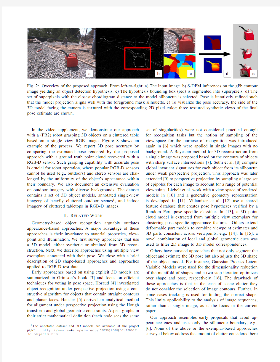
Fig.2:Overview of the proposed approach.From left-to-right:a)The input image.b)S-DPM inferences on the gPb contour image yielding an object detection hypothesis.c)The hypothesis bounding box(red)is segmented into superpixels.d)The set of superpixels with the closest chordiogram distance to the model silhouette is selected.Pose is iteratively re?ned such that the model projection aligns well with the foreground mask silhouette.e)To visualize the pose accuracy,the side of the 3D model facing the camera is textured with the corresponding2D pixel color;three textured synthetic views of the?nal pose estimate are shown.
In the video supplement,we demonstrate our approach with a(PR2)robot grasping3D objects on a cluttered table based on a single view RGB image.Figure8shows an example of the process.We report3D pose accuracy by comparing the estimated pose rendered by the proposed approach with a ground truth point cloud recovered with a RGB-D sensor.Such grasping capability with accurate pose is crucial for robot operation,where popular RGB-D sensors cannot be used(e.g.,outdoors)and stereo sensors are chal-lenged by the uniformity of the object’s appearance within their boundary.We also document an extensive evaluation on outdoor imagery with diverse backgrounds.The dataset contains a set of3D object models,annotated single-view imagery of heavily cluttered outdoor scenes1,and indoor imagery of cluttered tabletops in RGB-D images.
II.R ELATED W ORK
Geometry-based object recognition arguably outdates appearance-based approaches.A major advantage of these approaches is their invariance to material properties,view-point and illumination.We?rst survey approaches that use a3D model,either synthetic or obtained from3D recon-struction.Next,we describe approaches using multiple view exemplars annotated with their pose.We close with a brief description of2D shape-based approaches and approaches applied to RGB-D test data.
Early approaches based on using explicit3D models are summarized in Grimson’s book[3]and focus on ef?cient techniques for voting in pose space.Horaud[4]investigated object recognition under perspective projection using a con-structive algorithm for objects that contain straight contours and planar faces.Hausler[5]derived an analytical method for alignment under perspective projection using the Hough transform and global geometric constraints.Aspect graphs in their strict mathematical de?nition(each node sees the same 1The annotated dataset and3D models are available at the project page:https://www.wendangku.net/doc/ac14711380.html,/?menglong/outdoor-3d-objects.html set of singularities)were not considered practical enough for recognition tasks but the notion of sampling of the view-space for the purpose of recognition was introduced again in[6]which were applied in single images with no background.A Bayesian method for3D reconstruction from a single image was proposed based on the contours of objects with sharp surface intersections[7].Sethi et al.[8]compute global invariant signatures for each object from its silhouette under weak perspective projection.This approach was later extended[9]to perspective projection by sampling a large set of epipoles for each image to account for a range of potential viewpoints.Liebelt et al.work with a view space of rendered models in[10]and a generative geometry representation is developed in[11].Villamizar et al.[12]use a shared feature database that creates pose hypotheses veri?ed by a Random Fern pose speci?c classi?er.In[13],a3D point cloud model is extracted from multiple view exemplars for clustering pose speci?c appearance features.Others extend deformable part models to combine viewpoint estimates and 3D parts consistent across viewpoints,e.g.,[14].In[15],a novel combination of local and global geometric cues was used to?lter2D image to3D model correspondences. Others have pursued approaches that not only segment the object and estimate the3D pose but also adjusts the3D shape of the object model.For instance,Gaussian Process Latent Variable Models were used for the dimensionality reduction of the manifold of shapes and a two-step iteration optimizes over shape and pose,respectively[16].The drawback of these approaches is that in the case of scene clutter they do not consider the selection of image contours.Further,in some cases tracking is used for?nding the correct shape. This limits applicability to the analysis of image sequences, rather than a single image,as is the focus in the current paper.
Our approach resembles early proposals that avoid ap-pearance cues and uses only the silhouette boundary,e.g., [6].None of the above or the exemplar-based approaches surveyed below address the amount of clutter considered here
and in most cases the object of interest occupies a signi?cant portion of the?eld of view.
Early view exemplar-based approaches typically assume an orthographic projection model that simpli?es the analysis. Ullman[17]represented a3D object by a linear combina-tion of a small number of images enabling an alignment of the unknown object with a model by computing the coef?cients of the linear combination,and,thus,reducing the problem to2D.In[18],this approach was generalized to objects bounded by smooth surfaces,under orthographic projection,based on the estimation of curvature from three or?ve images.Much of the multiview object detector work based on discrete2D views(e.g.,[19])has been founded on successful approaches to single view object detection, e.g.,[1].Savarese and Fei-Fei[20]presented an approach for object categorization that combines appearance-based descriptors including the canonical view for each part,and transformations between parts.This approach reasons about 3D surfaces based on image appearance features.In[21], detection is achieved simultaneously with contour and pose selection using convex relaxation.Hsiao et al.[22]also use exemplars for feature correspondences and show that ambiguity should be resolved during hypothesis testing and not at the matching phase.A drawback of these approaches is their reliance on discriminative texture-based features that are hardly present for the types of textureless objects considered in the current paper.
As far as RGB-D training and test examples are concerned, the most general and representative approach is[23].Here, an object-pose tree structure was proposed that simultane-ously detects and selects the correct object category and instance,and re?nes the pose.In[24],a viewpoint feature histogram is proposed for detection and pose estimation. Several similar representations are now available in the Point Cloud Library(PCL)[25].We will not delve here into approaches that extract the target objects during scene parsing in RGB-D images but refer the reader to[26]and the citations therein.
The2D-shape descriptor,chordiogram[2],we use belongs to approaches based on the optimal assembly of image regions.Given an over-segmented image(i.e.,superpixels), these approaches determine a subset of spatially contiguous regions whose collective shape[2]or appearance[27]fea-tures optimize a particular similarity measure with respect to a given object model.An appealing property of region-based methods is that they specify the image domain where the object-related features are computed and thus avoid con-taminating objected-related measurements from background clutter.
III.T ECHNICAL APPROACH
An overview of the components of our approach is shown in Fig.2.3D models are acquired using a low-cost depth sensor(Sec.III-A).To detect an object robustly based only on shape information,the gPb contour detector[28]is applied to the RGB input imagery(Sec.III-B).Detected contours are fed into a parts-based object detector
trained Fig.3:Comparison of the two edge detection results on same image.(left-to-right)Input image,Canny edge and gPb, respectively.
on model silhouettes(Sec.III-C).Detection hypotheses are over-segmented and shape veri?cation simultaneously com-putes the foreground segments and reranks the hypotheses (Sec.III-E).Section III-D describes the shape descriptor used for shape veri?cation.The obtained object mask enables the application of an iterative3D pose re?nement algorithm to accurately recover the6-DOF object pose based on the initial coarse pose estimate rendered by the object detector(Sec. III-F).
A.3D model acquisition and rendering
3D CAD models have been shown to be very useful for object detection and pose estimation both in2D images and 3D point clouds.We utilize a low-cost RGB-D depth sensor and a dense surface reconstruction algorithm,KinectFusion [29],to ef?ciently reconstruct3D object models from the depth measurements of real objects.The3D object model is acquired on a turntable with the camera pointing in a?xed position.After the model is reconstructed with the scene,we manually remove the background and?ll holes in the model. To render object silhouettes from arbitrary poses,we synthesize a virtual camera at discretized viewpoints around the object center at a?xed distance.Each viewpoint is parameterized by the azimuth,a,elevation,e,and distance,d, of the camera relative to the object.Viewpoints are uniformly sampled on the viewsphere at a?xed distance and at every ten degrees for both the azimuth and elevation.
B.Image feature
Our approach to shape-based recognition bene?ts from recent advances in image contour detection.In unconstrained natural environments,the Canny edge detector[30]generally responds uniformly to both object occlusion boundaries and texture.One can falsely piece together the silhouette of a target object from a dense set of edge pixels.The state-of-the-art contour detection algorithm gPb[28]computes the likelihood of each pixel being an object contour and thus suppresses many edges due to texture/clutter.Figure3 shows an example of Canny edge detection and gPb on the same input https://www.wendangku.net/doc/ac14711380.html,pared to Canny edges,gPb suppresses ubiquitous edge responses from background clutter. Given detected contours in the image,we seek to localize the subset of contour pixels that best represent the object silhouette.We will show that for cluttered scenes,discrimi-native power is essential to achieve high recall with desired precision.
Fig.4:Spray bottle detection using S-DPM.(?rst row,left-to-right)Root appearance model,part appearance models centered at their respective anchor points and the quadratic deformation cost;brighter regions indicate larger penalty cost.(second row)Input image and detection response map of the spray-bottle;red,yellow and blue indicate large, intermediate and low detection responses,respectively.
C.Object detection
The Deformable Parts Model(DPM)[1]is arguably the most successful object detector to-date.DPM is a star-structured conditional random?eld(CRF),with a root part, F0,capturing the holistic appearance of the object and several parts(P0,...,P n)connected to the root where P i= (F i,v i,s i,a i,b i).Each model part has a default relative position(the anchor point),v i,with respect to the root position.Parts are also allowed to translate around the anchor point with a quadratic offset distance penalty,parameterized by the coef?cients a i and b i.The anchor points are learned from the training data and the scales of the root and parts, s i,are?xed.The detection score is de?ned as:
n
i=0F i·φ(H,p i)?n i=1a i·(?x i,?y i)+b i·(?x i2,?y i2),(1)
whereφ(H,p i)is the histogram of gradients(HOG)[31] feature extracted at image location p i,and(?x i,?y i)is the offset to the part anchor point with respect to the root position p0.At test time,the root and part model weights are each separately convolved with the HOG feature of the input image.Due to the star structure of the model,maximizing the above score function at each image location can be computed ef?ciently via dynamic programming.To deal with intra-class variation,DPM is generalized by composing several components,each trained on a subset of training instances of similar aspect ratio.We refer to[1]for more details. To simultaneously detect an object and coarsely estimate its pose from the edge map using only model silhouette shape information,we train a shape-aware modi?ed version of DPM,which we term S-DPM.Each component of the learned S-DPM corresponds to a coarse pose of the object. More speci?cally,the silhouettes of the synthetic views of the object are clustered into16discrete poses by grouping nearby viewpoints.A S-DPM component is trained based on the silhouettes of a coarse pose cluster used as positive training data and silhouettes of other poses and objects and random background edges used as negatives.Figure4 shows an example of a trained spray bottle model.During inference,each of the model components are evaluated on the input contour imagery and the hypotheses with a detection score above a threshold are retained.Detections of different components are combined via non-maximum suppression. This step retains high scoring detections and?lters out neighboring lower scoring ones whose corresponding2D bounding box overlaps with that of the local maximum by greater than50%(PASCAL criteria[32]).The coarse pose of the object is determined by the maximum scoring component at each image location.
D.Shape descriptor
We represent the holistic shape of each S-DPM detected object with the chordiogram descriptor[2].Given the ob-ject silhouette,this representation captures the distribution of geometric relationships(relative location and normals) between pairs of boundary edges,termed chords.Formally, the chordiogram is a K-dimensional histogram of all chord features on the boundary of a segmented object.A chord is a pair of points(p,q)on the boundary points.Chord feature d pq=(l pq,ψpq,θp?ψpq,θq?ψpq) is de?ned by chord vector length l pq,orientationψpq and normals θp andθq of the object boundary at p and q.The edge normal direction points towards the segment interior to distinguish the same edge with different foreground selection of bordering superpixels.Figure5shows two examples of chord features and their corresponding chordiogram feature bins when the bordering foreground superpixels differ.The chordiogram is translation invariant since it only relates the relative position of boundary pixels rather than the absolute position in the image.
E.Shape veri?cation for silhouette extraction
We use the chordiogram descriptor for two tasks:(i)to recover the object foreground mask(i.e.,the silhouette)for accurate3D pose estimation and(ii)to improve detection precision and recall by verifying that the shape of the foreground segmentation resembles the model mask.
The fact that S-DPM operates on HOG features provides ?exibility in dealing with contour extraction measurement noise and local shape variance due to pose variation.How-ever,S-DPM only outputs the detections of the object hypotheses rather than the exact location of the object contour.Even in the object hypothesis windows,the subset of edge pixels that correspond to the object silhouette is not apparent.In addition,contour-based object detection in cluttered scenes is susceptible to false detections caused by piecing together irrelevant contours.
Left:Example of a con?guration Right:A chordiogram d of the length and orientation an be decomposed as the sum ords (bottom
right).E BoSS (s )=match (s,m )+group (s )(1)ollowing,we describe our shape representation and s of the model.ordiograms as Shape Representation
valuate the similarity between a ?gure/ground seg-on and the model mask we use a global
boundary-hape descriptor,called the chordiogram .It is in-y the Gestalt principle postulating that shape is per-s whole [18],as well as by the success of contour-hape descriptors [1].
e?ne a chordiogram,consider all possible pairs of y edges of a segmented object,called chords.Each aptures the geometric con?guration of two bound-es,and their distribution can be used to describe
bal shape.More precisely,for each chord (p,q ),?guration is described as:the length l pq and the on pq of the vector connecting p and q as well
orientations ?p and ?q of the normals to the seg-on boundary at p and q (see Fig.2,left).The lat-ntations are de?ned such that they point towards ct interior.Note that in this way we capture not e boundary but also the object interior.Thus,the
ation features of a chord (p,q )can be written as:?p pq ,?q pq ,l pq , pq )T ,where the normal ori-
3.The top 2principal components of chord using PCA for objects in the ETHZ Shape 5).(We omit the class ’Applelogos’for the sa ).
invariant.The descriptor is also inspired by C which captures topological properties of set of Another important difference is that we cap tour orientation relative to object interior.O boundary normals with respect to the interio to better discrimination,for example,between convex structures (con?gurations f pq and f p 0q 0in Fig.2),which otherwise would be indistingu discriminative power can be seen on the right s where objects of four different types are well s ing chordiograms,provided we compute it o objects.If,however,we use all image con the object bounding box,we obtain cluttered (Fig.3,left),which are much harder to separate vates the coupling of the chordiogram with ?g tation,as explained next.This coupling allow descriptor support which covers the whole obj descriptor is used globally.3.2.Boundary Structure Matching
The matching term in Eq.(1)compares the c of the model and an image segmentation.T the matching model,we need to express the d a function of the object segmentation s .It wi ful to provide an equivalent de?nition to Eq.(the contribution of a chord (p,q )to the desc noted by a chord descriptors d pq 2{0,1}K :
iff f pq 2bin (k ).Then Eq.(2)can be expres ear function of the chord contributions:d =
p
q
p’
q’
Fig.5:Chordiogram construction.image on the left denotes the object.Gray highlighted superpixels under consideration.p q
,the features,f pq and f p q
,fall into different bins of the histogram,i.e.,the chordiogram shown on the right.At each boundary point,the foreground selection of bordering superpixels de?nes the normal direction.
To recover exact object contour pixel locations
and reduce false positives,an additional shape matching step is required on top of the object hypotheses.Here,we propose using the collective shape of a subset of superpixels within each
hypothesis region to verify the presence of an object.
For each detection hypothesis region,superpixels are
computed directly from gPb [28].Searching over the entire space of superpixel subsets for the optimal match between the collective shape of the superpixels and the object model
is combinatorial and impractical.Instead,we use a greedy
algorithm to ef?ciently perform the search.In practice,with limited superpixels to select from,our greedy approach
recovers the correct region with high probability.Figure
6shows example results of shape veri?cation.The greedy algorithm begins with a set of connected superpixels as a
seed region and greedily searches over adjacent superpixels,
picking the superpixel that yields the smallest χ2distance to the chordiogram of model silhouette.Intuitively,if we have
a set of superpixels forming a large portion of the object
with a few missing pieces,adding these pieces yields the best score.The initial seeds are formed by choosing all triplets of
adjacent superpixels,and limiting examination to the top ?ve
seeds that yield the smallest χ2
distance.The connectivity graph of superpixels is a planar graph with limited node
degrees.The complexity of ?nding triplets in such a planar graph is O (N log N )in the number of nodes.
Once the correct foreground superpixels are selected,the detection bounding box is re-cropped to re?ect the recovered
foreground mask.Empirically,this cropping step yields a
better localization of the detection result over the S-DPM,as measured in terms of precision and recall,see Sec.IV
Edges of the foreground mask are extracted and used in the
subsequent processing stage for accurate 6-DoF continuous pose estimation.
Fig.6:Shape descriptor-based veri?cation examples.(left-to-right)Detection hypothesis window of the object,superpixel
over-segmentation of the hypothesis region,visualization of the coarse object pose from the object detector and selected foreground mask.
F .Pose re?nement
Robotic grasping requires an accurate estimate of an
object’s 3D pose.To improve upon the coarse pose estimate provided by the S-DPM,we perform a ?nal iterative pose re?nement step to recover the full continuous 6-DoF pose.
This step is restricted to the region of the veri?ed superpixel
mask.Our iterative re?nement process consists of two steps:
(i)determining the correspondence between the projected occluding boundary of the 3D model and the contour points along object segmentation mask,and (ii)estimating an
optimal object pose based on the correspondences.The contour correspondences are estimated using dynamic programming (DP)to ensure local matching smoothness.Given the initial (coarse)pose output from the object detec-
tion stage,the 3D object model is rendered to the image and its corresponding projected occluding boundary is extracted.Each point on the contour is represented by a descriptor capturing close-range shape information.The 31-dimensional
contour descriptor includes the gradient orientation of a con-tour point (the central point)and the gradient orientations of the nearest 15points on each side of the central point along
the contour.The gradient orientation of the central point is subtracted from all elements of the descriptor,which gives in-plane rotation invariance.The matching cost between each
pair is set to be the l 2distance of the feature descriptor extracted at each point.DP is then used to establish the correspondences between contour points.
Fig.7:Representative images from the introduced outdoor dataset.The dataset was captured using a ground robot and includes diverse terrains,e.g.,rocks,sand and grass,with illumination changes.Portions of the terrain are non-?at. Objects are scattered around the scene and typically do not occupy a major portion of the scene.
To estimate the re?ned pose we use the motion?eld equation[33]:
u(x,y)=1
Z
(xt z?t x)+ωx(xy)?ωy(x2+1)+ωz(y)
v(x,y)=1
Z
(yt z?t y)?ωx(y2+1)?ωy(xy)+ωz(x),
where u(x,y),v(x,y)denote the horizontal and vertical components of the displacement vectors,respectively,be-tween the model and matched image contour points,com-puted by DP,Z(x,y)denotes the depth of the3D model point for the current pose estimate and the Euler angles (ωx,ωy,ωz)and3D translation vector(t x,t y,t z)denote the (locally)optimal motion of the object yielding the re?ned pose.The motion update of the current pose is recovered using least squares.This procedure is applied iteratively until convergence.In practice,we usually observe fast conver-gence with only three to?ve iterations.The running time of the pose re?nement is about one second on an Intel2.4GHz i7CPU.
IV.E XPERIMENTS
Outdoor detection evaluation We introduce a challenging outdoor dataset for3D object detection containing heavy background clutter.This dataset was collected from a moving robot and consists of eight sequences containing a total of3403test images;the dimensions of each image are 512×386.Figure7shows a set of representative imagery from the introduced dataset.The scenes contain a variety of terrains(e.g.,grass,rock,sand,and wood)observed under various illumination conditions.The dataset represents the task of a robot navigating a complex environment and searching for objects of interest.The objects of interest are mostly comprised of textureless daily equipment,such as a watering pot,gas tank,watering can,spray bottle,dust pan, and liquid container.For each frame,2D bounding boxes that tightly outline each object are provided.Further,the dataset includes the corresponding3D model?les used in our empirical evaluation.
On the outdoor dataset,we performed a shape-based object detection evaluation.We compared four methods,DOT[34], S-DPM with only the root model,full S-DPM with root and parts,and the full S-DPM plus shape veri?cation(proposed approach),on a detection task on the introduced dataset.Both DOT and S-DPM used the same training instances from Sec. III-A with a slight difference.For S-DPM,we trained one model component for each of16discrete poses.For DOT, we used the same quantization of the viewsphere but trained with10different depths ranging from close to far in the scene.During testing,S-DPM is run on different scales by building an image pyramid.The input to both methods were the same gPb thresholded images.In all our experiments, the threshold is set to40(gPb responses range between0 and255),where edges with responses below the threshold were suppressed.The default parameters of gPb were used. We did not observe a noticeable difference in the detection and pose estimate accuracy with varying the gPb parameter settings.
Table III shows a comparison of the average precision for detection on the outdoor dataset.The proposed approach consisting of the full S-DPM plus shape veri?cation achieves the best mean average precision.It demonstrates that using shape veri?cation improves detection due to the re?nement of the bounding box to re?ect the recovered silhouette.Full S-DPM outperforms both the root only S-DPM and DOT.This shows the bene?t of the underlying?exibility in S-DPM. Table top evaluation We evaluated our pose re?nement approach under two settings.First,we recorded an indoor RGB-D dataset,with multiple objects on a table,from a head mounted Kinect on a PR2robot.The RGB-D data is used as ground truth.We evaluated using three objects, watering can,gas tank,watering pot,placed at two different distances from the robot on the table and two different poses for each distance.For each scene,the target object was detected among all objects on the table and segmented using shape veri?cation,and then the6-DoF pose was estimated,as described in Sec.III-F.The model point cloud was projected into the scene and Iterative Closest Point(ICP)[35]was performed between the model point cloud and the Kinect point cloud.We report ICP errors for both rotation and translation in Tables I and II,resp.Errors in the rotations and translations are small for different angles and different depth. Translation errors in the X and Y directions are smaller than in Z direction.Since Z is the depth direction,it is most affected by the3D model acquisition and robot calibration. Both measurements show our method is robust and suitable for grasping task.
In addition,using the object pose estimated from our approach,we demonstrate with a PR2robot successful
watering pot gas tank watering can spray bottle dust pan liquid container average AP S-DPM full+shape0.6860.6450.5230.5150.4290.5060.5507 S-DPM full0.6880.6100.5470.5070.3870.5090.5413 S-DPM root only0.4690.5350.4330.4360.2950.4360.4340 DOT0.4070.4120.3400.0890.1110.1880.2578 TABLE III:Average precision on the introduced outdoor dataset.
Estimated Rotation Error
Roll Pitch Yaw Roll Pitch Yaw
dist1 1.6548.44-145.370.99 3.57-1.63 watering 5.5050.73-22.37-3.20-3.92-0.07
can dist2-4.3341.9348.78-3.20-3.92-0.07
2.4449.60-54.82-0.12 1.95-1.92
dist1-0.4359.20-73.00-1.25-0.28 1.36 watering0.6951.90156.86-1.82-0.63-3.48
pot dist2-10.4366.9338.28-1.078-6.67-2.43
-0.63352.24-131.94-0.21 1.14-0.88
dist1-0.1550.58-136.17 1.43 2.73-4.58 gas 2.8450.15-51.15-2.63 3.20 2.79
tank dist2-2.4448.24129.43-3.570.02-2.14
-7.4045.22109.90-1.55-1.79-1.03 TABLE I:Estimated absolute rotation of the object and error in degrees.
Estimated Translation Error
X Y Z X Y Z
dist1-46.5-82.3-1023.6-1.14-0.7-2.8 watering-57.1-86.4-1023.2-1.2 2.8-7.2
can dist2-85.1183.2-1182.9 3.6 3.6 4.8
-114.9186.0-1200.3 4.5 2.2-5.1
dist116.4-154.0-1020.9 2.8 1.00.06 watering-117.6-112.4-1028.30.40.2 2.2
pot dist2-6.832.7-1051.2 2.0-2.9-3.5
-106.5-6.6-1053.1-0.5-0.2-1.9
dist1-23.821.2-1061.2-1.8-0.9-3.2 gas19.5-116.0-958.8-0.4 1.7-3.2
tank dist2-77.0 6.7-1064.60.4-0.9-2.0
-111.3178.9-1200.80.6-0.4-1.4 TABLE II:Estimated absolute translation of the object and error in centimeters.
detections and grasps of various objects from a cluttered table.In Fig.8,we show qualitative results of the PR2 successfully grasping various objects on a cluttered table.
V.C ONCLUSION
We presented an integrated approach for detecting and lo-calizing3D objects using pure geometric information derived from a database of3D models.We create an initial set of hypotheses with a state-of-the-art parts-based model trained on clusters of poses.Detection hypotheses are segmented and reranked by matching subsets of superpixels with model boundary silhouettes using the chordiogram descriptor.The resulting segmentation enables the re?nement of3D pose in a small number of steps.Due to the holistic nature of the chordiogram-based superpixel selection,our approach is resistant to clutter.We demonstrate the grasps of texture-less objects in dif?cult cluttered environments in the video supplement.
Acknowledgment Financial support through the follow-ing grants NSF-IIP-0742304,NSF-OIA-1028009,ARL MAST CTA W911NF-08-2-0004,and ARL Robotics CTA W911NF-10-2-0016,NSF-DGE-0966142,and NSF-IIS-1317788is gratefully acknowledged.
R EFERENCES
[1]P.Felzenszwalb,R.Girshick,D.McAllester,and D.Ramanan,“Object
detection with discriminatively trained part-based models,”PAMI, vol.32,no.9,pp.1627–1645,2010.
[2] A.Toshev,B.Taskar,and K.Daniilidis,“Shape-based object detection
via boundary structure segmentation,”IJCV,vol.99,no.2,pp.123–146,2012.
[3]W.Grimson,Object recognition by computer:The role of geometric
constraints.Cambridge,MA:The MIT Press,1990.
[4]R.Horaud,“New methods for matching3-D objects with single
perspective views,”PAMI,vol.9,no.3,pp.401–412,May1987. [5]G.H¨a usler and D.Ritter,“Feature-based object recognition and
localization in3D-space,using a single video image,”CVIU,vol.73, no.1,pp.64–81,January1999.
[6] C.Cyr and B.Kimia,“3D Object Recognition Using Shape Similarity-
Based Aspect Graph,”in ICCV,2001,pp.254–261.
[7] F.Han and S.Zhu,“Bayesian reconstruction of3D shapes and scenes
from a single image,”in Int.Workshop on High Level Knowledge in 3D Modeling and Motion,2003.
[8] A.Sethi,D.Renaudie,D.Kriegman,and J.Ponce,“Curve and surface
duals and the recognition of curved3D objects from their silhouettes,”
IJCV,vol.58,no.1,pp.73–86,June2004.
[9]https://www.wendangku.net/doc/ac14711380.html,zebnik, A.Sethi, C.Schmid, D.Kriegman,J.Ponce,and
M.Hebert,“On pencils of tangent planes and the recognition of smooth3D shapes from silhouettes,”in ECCV,2002,pp.III:651–665.
[10]J.Liebelt,C.Schmid,and K.Schertler,“Viewpoint-independent object
class detection using3D Feature Maps,”in CVPR,2008,pp.1–8. [11]J.Liebelt and C.Schmid,“Multi-view object class detection with a
3D geometric model,”in CVPR,2010,pp.1688–1695.
[12]M.Villamizar,H.Grabner,J.Andrade-Cetto,A.Sanfeliu,L.Van Gool,
F.Moreno-Noguer,and K.Leuven,“Ef?cient3D object detection
using multiple pose-speci?c classi?ers,”in BMVC,2011.
[13] D.Glasner,S.Vitaladevuni,and R.Basri,“Contour-based joint
clustering of multiple segmentations,”in CVPR,2011,pp.2385–2392.
[14] B.Pepik,M.Stark,P.Gehler,and B.Schiele,“Teaching3D geometry
to deformable part models,”in CVPR,2012,pp.3362–3369. [15]Q.Hao,R.Cai,Z.Li,L.Zhang,Y.Pang,F.Wu,and Y.Rui,“Ef?cient
2D-to-3D correspondence?ltering for scalable3d object recognition,”
in CVPR,2013.
[16]V.A.Prisacariu,A.V.Segal,and I.Reid,“Simultaneous monocular
2D segmentation,3D pose recovery and3D reconstruction,”in ACCV.
Springer,2013,pp.593–606.
[17]S.Ullman and R.Basri,“Recognition by linear combinations of
models,”PAMI,vol.13,pp.992–1006,1991.
[18]R.Basri and S.Ullman,“The alignment of objects with smooth
surfaces,”CVGIP,vol.57,no.3,pp.331–345,May1993.
[19] C.Gu and X.Ren,“Discriminative mixture-of-templates for viewpoint
classi?cation,”in ECCV,2010,pp.V:408–421.
[20]S.Savarese and L.Fei-Fei,“3D generic object categorization,local-
ization and pose estimation,”in ICCV,2007,pp.1–8.
[21]N.Payet and S.Todorovic,“From contours to3D object detection and
pose estimation,”in ICCV,2011,pp.983–990.
[22] E.Hsiao,A.Collet,and M.Hebert,“Making speci?c features less
discriminative to improve point-based3D object recognition,”in CVPR.IEEE,2010,pp.2653–2660.
[23]https://www.wendangku.net/doc/ac14711380.html,i,L.Bo,X.Ren,and D.Fox,“A scalable tree-based approach
for joint object and pose recognition,”in AAAI,2011.
[24]R.Rusu,G.Bradski,R.Thibaux,and J.Hsu,“Fast3D recognition
and pose using the viewpoint feature histogram,”in IROS,2010,pp.
2155–2162.
Fig.8:PR2grasping process for two example input images.Top panel for gas tank and bottom for dust pan.a)S-DPM detection bounding boxes ordered by the detection score in decreasing order.b)Corresponding pose output from S-DPM for each detection.c)Segmentation of top scored detection window.d)Foreground mask selected by shape veri?cation.e)Three iterations in pose re?nement,alignments (shown in color)between curves are computed using DP.f)Visualization of PR2model with the Kinect point cloud.Notice that the estimated model given in light green is well aligned with the point cloud.Grasping points are indicated by arrow.g)Another view of the same scene.
[25]R.B.Rusu and S.Cousins,“3D is here:Point cloud library (PCL),”
in ICRA ,2011,pp.1–4.
[26]H.Koppula, A.Anand,T.Joachims,and A.Saxena,“Semantic
labeling of 3D point clouds for indoor scenes,”in NIPS ,2011.
[27]S.Vijayanarasimhan and K.Grauman,“Ef?cient region search for
object detection,”in CVPR ,2011,pp.1401–1408.
[28]P.Arbelaez,M.Maire,C.Fowlkes,and J.Malik,“Contour detection
and hierarchical image segmentation,”PAMI ,vol.33,no.5,pp.898–916,2011.
[29]S.Izadi,R.Newcombe, D.Kim,O.Hilliges, D.Molyneaux,
S.Hodges,P.Kohli,J.Shotton,A.Davison,and A.Fitzgibbon,“Kinectfusion:real-time dynamic 3D surface reconstruction and in-teraction,”in ACM SIGGRAPH ,vol.23,2011.
[30]J.Canny,“A computational approach to edge detection,”PAMI ,no.6,
pp.679–698,1986.
[31]N.Dalal and B.Triggs,“Histograms of oriented gradients for human detection,”in CVPR ,2005,pp.I:886–893.
[32]M.Everingham,L.Van Gool,C.K.I.Williams,J.Winn,and A.Zisserman,“The pascal visual object classes (voc)challenge,”IJCV ,vol.88,no.2,pp.303–338,June 2010.
[33] B.K.P.Horn,Robot Vision .the MIT Press,1986.
[34]S.Hinterstoisser,V .Lepetit,S.Ilic,P.Fua,and N.Navab,“Dominant orientation templates for real-time detection of texture-less objects,”in CVPR ,2010,pp.2257–2264.
[35]
P.Besl and N.McKay,“A method for registration of 3-D shapes,”PAMI ,vol.14,no.2,pp.239–256,February 1992.
真正实现C语言绘制数学函数图像
用C语言画函数图像 横纵坐标单位长度比校正(3:5) 真正的余弦函数 #include
a[i] = a[i - 1] + 0.01; b[i] = cos(a[i]); } int A[500],B[500]; for (i = 0; i < n; i++) { //printf("sin(%f)=%f\n", a[i], b[i]); a[i] = 100 * a[i]; b[i] = 55 * b[i]; A[i] = sishewuru(a[i]); B[i] = sishewuru(b[i])+60; //printf("sin(%d)=%d\n", A[i], B[i]); } for ( i = 100; i >=0; i--) { for ( j = 0; j < n; j++) { if (i==B[j]) { printf("*"); } else { printf(" "); } } printf("\n"); } } int sishewuru(float a) { int m; if (a-floor(a)<0.5) { m = a; return m; } else { m = a + 1; return m; } }
1.调节输出框大小,字符显示大小 2.确定函数的定义域 3.确定定义域上的步长 4.计算函数值 5.确定函数值放大系数 6.确定定义域恰好落在显示的区间内 7.确定坐标的单位长度与字符实际长度之间的换算关系 8.确定打点的顺序与坐标的关系 定义域在),(ππ-的正弦函数图像 定义域在),(ππ-的正切函数图像
Matlab画函数图像
用Matlab画函数图像 一、螺旋线 1.静态螺旋线 a=0:0.1:20*pi; h=plot3(a.*cos(a),a.*sin(a),2.*a,'b','linewidth',2); axis([-50,50,-50,50,0,150]); grid on set(h,'erasemode','none','markersize',22); xlabel('x轴');ylabel('y轴');zlabel('z轴'); title('静态螺旋线'); 2.动态螺旋线 t=0:0.1:10*pi; i=1; h=plot3(sin(t(i)),cos(t(i)),t(i),'*','erasemode','none'); grid on axis([-2 2 -2 2 0 35]) for i=2:length(t)
set(h,'xdata',sin(t(i)),'ydata',cos(t(i)),'zdata',t(i)); drawnow pause(0.01) end title('动态螺旋线'); (图略) 3.圆柱螺旋线 t=0:0.1:10*pi; x=r.*cos(t); y=r.*sin(t); z=t; plot3(x,y,z,'h','linewidth',2); grid on axis('square') xlabel('x轴');ylabel('y轴');zlabel('z轴'); title('圆柱螺旋线') 二、旋转抛物面
b=0:0.2:2*pi; [X,Y]=meshgrid(-6:0.1:6); Z=(X.^2+Y.^2)./4; meshc(X,Y,Z); axis('square') xlabel('x轴');ylabel('y轴');zlabel('z轴'); title('旋转抛物面') 或直接用:ezsurfc('(X.^2+Y.^2)./4') 三、椭圆柱面 load clown ezsurf('(2*cos(u))','4*sin(u)','v',[0,2*pi,0,2*pi]) view(-105,40) %视角处理 shading interp %灯光处理 colormap(map) %颜色处理 grid on %添加网格线 axis equal %使x,y轴比例一致 xlabel('x轴');ylabel('y轴');zlabel('z轴'); %添加坐标轴说明title('椭圆柱面') %添加标题
怎样在Word文档中绘制函数图像
怎样在Word文档中绘制函数图像 摘要: Microsoft office word 是应用最广泛的办公软件之一,它具有强大的文字、表格、图形等处理功能,为用户提供了很大方便。然而,要用它进行函数图像绘制和编辑却非常困难。使很多用户(比如数学教师)编写教案、学案、考试试卷等含有函数图像的文档成为一大难题。 笔者经过多年的研究和探索,尝试着利用Word的Visual Basic 编辑器,实验性地开发了一个“图像工具”软件,使函数图像的绘制和编辑变得简单易行。使用过程中感觉良好,与大家分享,希望能起到抛砖引玉的作用。 一、绘制函数图像的困难与尝试 作为一个从事数学教学多年的教师,经常用Microsoft office word软件编写教案、学案、考试试卷等教学资料。每当用到函数图像时就感到非常困难,因为word中没有针对函数图像的功能。采取的办法通常是从其它资料中复制粘贴、扫描现成的图像、用专用绘图软件(如几何画板)绘制,再插入到文档中。这样带来的问题是:第一不方便,第二兼容性不好,插入后就变成了图片格式,编辑修改困难,很难精确实现自己的意图。 于是就尝试着利用Word的Visual Basic 编辑器,编写了一个函数图像绘制工具。它不但能在坐标系中精确的绘制常用函数的图像,而且能演示图像的绘制过程,反应y随x变化而变化的规律与特点,更好的揭示函数图像的实质,也能够演示图像变换,反应函数图像与函数解析式的内在联系。在方便编辑含有函数图像的教学资料的同时,也能让学生更好的理解函数图像的实质,提高教学效果。 二、图像工具的应用举例
由于编写了安装和卸载程序,使得图像工具的安装和卸载实现了一键完成,用户不需要有Visual Basic 编程基础,安装完成后word (以word 2003为例)的绘图工具栏如图1所示,添加了一个“插入图像”按钮,单击该按钮就可以调用 图像工具了。 下面以正弦型函数为例介绍图像工具的应用。 1、将光标移到要插入图像的位置,单击“插入图像”按钮,窗口将弹出如图2所示的窗体。 2、在窗体中选择“正弦 型”函数,勾选“附加坐标系”,参数ω设为1/2(也可用小数0.5),右界设为4,其他采用缺省值,单击“设置完成”,右边正弦型函数的解析式将变成y = sin(0.5x ),同时改变颜色(如果参数中含有非法数据,将给出错误提示),再单 图 1 图 2
用计算机绘制函数图像
用计算机绘制函数图像 利用计算机软件可以便捷、迅速地绘制各种函数图像。不同的计算机软件绘制函数图像的具体操作不尽相同,但都是基于我们熟悉的描点作图。即给子变量赋值,用计算法则算出相应的函数值,再由这些对应值生成一系列的点,最后连接这些点描绘出函数图像。下面以Excel 和《几何画板》为例,介绍用计算机软件作函数图像的方法。 1.用“Excel ”绘制函数3 y x =的图像 (1) 打开Excel ,在A 列输入自变量x 的值; (2) 把光标移到B 列,在编辑框输入计算法则“=POWER (A :A ,3)”,回车,在B 列 生成相应的函数值,如图1所示; (3) 选中数据区域A 、B 列,执行“插入→图表”命令,在“图表类型”中选择“XY 散点”,根据需要在“子图表类型”中选择其一。然后按照对话框中的提示,完成制图操作,就可得到如图2所示的函数3y x =的图像。 图1 图2 2.用《几何画板》绘制函数2(0)y bx b =≠的图像 (1) 打开几何画板,通过执行“构造/平行线”和“构造/线段”,生成平行于x 轴的 线段AB ,将A 固定于y 轴,B 为动点,选中B 点,执行“度量/横坐标”选项,画板上显示的点B 的横坐标B x 就是参数b 的值。 (2) 执行“图表/新建函数”,在对话框内输入函数表达式“*^2B x x ”,执行“图表 /绘制新函数”,即生成函数图像,如图3。
图3 图4 当你左右移动B 点的位置时,函数2(0)y bx b =≠就会“动”起来,如图4,如果有条件,请你绘制函数2(0)y ax bx c a =++≠的图像,并探究系数a 、b 、c 对函数图象的影响。
绘制函数图象的五种技法
绘制函数图象的五种技法 如今的社会真的是靠脸吃饭的么?小编我却不以为然,还是觉得靠技术吃饭比较重要,技术不压身!现代教学是多媒体教学,那就离不开教学软件的支撑,几何画板就是其中之一。在用几何画板辅助数学教学的过程中,常常涉及到函数图象的绘制。熟练掌握绘制函数图象的方法,对提高数学教学效率很有帮助。下面小编通过实例来系统总结绘制函数图象的五种技法,如果你get以下几个新技能,离超级学霸就不远啦! 一、直接法 例1 画函数y=sinx在R上的图象。 操作步骤:单击“图表”菜单下“绘制新函数”f(x)=sinx(如图1)。 二、轨迹法 例2 画函数y=(1/4)x^2在区间[-2,3]上的图象。 操作步骤: (1)单击“绘图”菜单下“绘制点”C(-2,0),D(3,0),构造线段CD;
(2)选中线段CD,单击“构造”菜单下“线段上的点”构造点E; (3)选中点E,单击“度量”菜单下“横坐标”得点E的横坐标xE; (4)单击“数据”菜单下“计算”,计算y值; (5)依次选中xE、y值,单击“绘图”菜单下“绘制(x,y)”,得点F; (6)选中点E与F,单击“构造”菜单下“轨迹”,得函数在区间[-2,3]的图象(如图2)。 三、参数法 例3 绘制二次函数y=-x2+2x+3的图象。 操作步骤: (1)单击“数据”菜单下“新建参数”a=-1,b=2,c=3; (2)单击“绘图”菜单下“绘制新函数”f(x)= =-x2+2x+3(如图3)。
改变参数a、b、c的值(可在选中后按“+”或“-”键),可以动态地探索与发现抛物线的开口方向、顶点坐标和对称轴的变化过程. 四、辅助函数法 例4画下面函数的图象。 操作步骤: (1)单击“数据”菜单下“新建函数”f(x)=sinx,g(x)=cosx; (2)单击“绘图”菜单下“绘制新函数”。(如图4)
用C++实现数学函数图形绘制(含源文件)
用VC++实现数学函数图形绘制 Use the VC++ to realize drawing figures of mathematic functions 摘要 Visual C++(以下简称VC++)是面向对象与可视化软件开发工具中比较成熟的一类。MFC是VC++中直接由Microsoft提供的类库,它集成了大量已定义好的类,我们可以根据需要,调用相应类,或根据需要自定义类。正是基于MFC 的这种特性,我们试图设计出具有封装性、独立性的功能模块------函数数据生成模块,函数曲线输出模块,模块之间的桥梁是由模板类CArray派生的CPoint 类数组充当的。函数数据生成模块用来实现对函数的设置并获得采样点,数组得到采样点数据并将其传递到输出模块中。从整体来看,实现了各程序模块的独立性,使得在函数模块中可任意添加、删除函数,可使用不同的DC和GDI,可实现不同的输出方式,整个工程在函数绘图功能上是无限扩展的。经过反复的调试和检验,我们实现了预期目标。我们的主要目的是尝试VC++在数学函数绘图方面的功能和应用。这是对VC++的探索,也是对数学函数绘图多样化的尝试。 关键字 数学函数图形绘制模板数组三次样条
【Abstract】 Visual C++ is one of the object oriented and visual software developer ,which is more mature than others . MFC is a class warehouse which is supplied by Microsoft ,and it contains a great deal of defined classes .we can transfer the corresponded class if necessary ,or give a fresh definition according our needs . Exactly based on MFC this kind of character, we try to design out the function mold which have the function to pack the class and be independent ------Mold for creating Function data, Mold for outputting the function curve, mold piece of born mold piece be sent by Cpoint Array rared by template CArray.The first mold is to make out sets for the function and get data we need which will be sent to the defined array,so now the array have the data that is to be got by the second mold.From whole project,we can see the independence of each mold,and exactly we may increase and decrease functions if necessary,we even can use different DC and GDI to realize the customed exportation method by which we can have a new view of the function curve. So, the function of the project can be extended freely.after repeatedly debugging and examining,we achieve our purpose.The most important thing we are trying is to find a way to connect the VC++ and the figures of mathmetic functions.This is not only a exploration to VC++,but also a attempt for realizing diversifing the mathmetic functions. 【Key words】 Mathematic functions drawingfigures template array tripline
描点法画函数图象的一般步骤
一.选择题 1.下列各点在函数2 y x -= 的图象上的是() A.(-2,1); B.(0,-2); C.(1,2); D.(2,-2) 答案:A 2.如图,下列四种表示方式中,能表示变量y 是x 的函数的有() A.1个; B.2个; C.3个; D.4个 答案:B 3.已知点A (2,3)在函数y=mx 2-x+1的图象上,则m 等于() A.1; B.-1; C.2; D.-2 答案:A 4.若点(m ,n )在函数y=2x+1的图象上,则2m-n 的值是() A.2; B.-2; C.1; D.-1 答案:D 5.如图,在平面直角坐标系中,四边形OABC 是菱形,点C 的坐标为(4,0),∠AOC=60°,垂直于x 轴的直线l 从y 轴出发,沿x 轴正方向以每秒1个单位长度的速度向右平移,设直线l 与菱形OABC 的两边分别交于点M ,N (点M 在点N 的上方),若△OMN 的面积为S ,直线l 的运动时间为t 秒(0≤t ≤4),则能大致反映S 与t 的函数关系的图象是()
答案:C 6.如图,在平面直角坐标系中,点B(1,1),半径为1、圆心角为90°的扇形外周有一动点P,沿A→B→C→A运动一圈,则点P的纵坐标y随点P走过的路程s之间的函数关系用图象表示大致是() 答案:C 7.甲、乙两人在一次赛跑中,路程s与时间t的关系如图所示(实线为甲的路程与时间的关系图象,虚线为乙的路程与时间的关系图象),小王根据图象得到如下四个信息,其中错误的是()
A.这是一次1500米赛跑; B.甲,乙两人中先到达终点的是乙; C.甲,乙同时起跑;D.甲在这次赛跑中的速度为5米/秒 答案:C 8.某电信部门为了鼓励固定电话消费,推出新的优惠套餐:月租费10元;每月拔打市内电话在120分钟内时,每分钟收费0.2元,超过120分钟的每分钟收费0.1元;不足1分钟时按1分钟计费.则某用户一个月的市内电话费用y(元)与拔打时间t(分钟)的函数关系用图象表示正确的是() 答案:B 9.三峡工程在6月1日至6月10日下闸蓄水期间,水库水位由106米升至135米,高峡平湖初现人间,假设水库水位匀速上升,那么下列图象中,能正确反映这10天水位h(米)随时间t(天)变化的是() 答案:B
19.1.2函数的图像(第一课时)
19.1.2函数的图象
[师]好!如果我们在直角坐标系中,将你所填表格中的自变量x及对应 的函数值S当作一个点的横坐标与纵坐标,即可在坐标系中得到一些点.大家思考一下,表示x与S的对应关系的点有多少个??如果全在坐标中指出的话是什么样子?可以讨论一下,然后发表你们的看法,建议大家不妨动手画画看. [生]这样的点有无数多个,如果全描出来太麻烦,也不可能.我们只能 描出其中一部分,然后想象出其他点的位置,用光滑曲线连接起来. [师]很好!这样我们就得到了一幅表示S与x关系的图.图中每个点都代表x的值与S的值的一种对应关系.如点(2,4)表示x=2时S=4.一般地,对于一个函数,如果把自变量与函数的每对对应值分别作为点的横、纵坐标,那么坐标平面内由这些点组成的图形,就是这个函数的图象(graph).?上图中的曲线即为函数S=x2(x>0)的图象. 函数图象可以数形结合地研究函数,给我们带来便利. [活动一] 活动内容设计: 下图是自动测温仪记录的图象,?它反映了北京的春季某天气温T如何 随时间t的变化而变化.你从图象中得到了哪些信息? 如有条件,你可以用带有温度探头的计算机(器),测试、记录温度和绘制表示温度变化的图象. 活动设计意图:
2.体会图象的直观性、优越性. 3.提高对图象的分析能力、认识水平. 4.掌握函数变化规律. 教师活动: 引导学生从两个变量的对应关系上认识函数,体会函数意义;可以指导 学生找出一天内最高、最低气温及时间;在某些时间段的变化趋势;认识图象的直观性及优缺点;总结变化规律……. 学生活动: 在教师引导下,积极探寻,合作探究,归纳总结. 活动结论: 1.一天中每时刻t都有唯一的气温T与之对应.可以认为,气温T是时间t的函数. 2.这天中凌晨4时气温最低为-3℃,14时气温最高为8℃. 3.从0时至4时气温呈下降状态,即温度随时间的增加而下降.从4 时至14?时气温呈上升状态,从14时至24时气温又呈下降状态.4.我们可以从图象中直观看出一天中气温变化情况及任一时刻的气温大约是多少. 5.如果长期观察这样的气温图象,我们就能得到更多信息,掌握更多 气温变化规律. [活动二] 活动内容设计: 下图反映的过程是小明从家去菜地浇水,又去玉米地锄草,然后回家.? 其中x表示时间,y表示小明离他家的距离. 根据图象回答下列问题: 1.菜地离小明家多远?小明走到菜地用了多少时间? 2.小明给菜地浇水用了多少时间? 3.菜地离玉米地多远?小明从菜地到玉米地用了多少时间?
如何用Excel画出复杂函数图象
Excel应用实例:轻松画出复杂的函数曲线 目标:教您轻松画好一条复杂的函数曲线。 实例:给出了一个函数式所对应的曲线的例子。 难点分析: 一些教师会遇到画函数曲线的问题吧!如果想快速准确地绘制一条函数曲线,可以借助EXCEL的图表功能,它能使您画的曲线既标准又漂亮。您一定会问,是不是很难学呀?其实一点儿也不难,不信您就跟我试一试。 以绘制y=|lg(6+x^3)|的曲线为例,其方法如下: 1) 自变量的输入 在某张空白的工作表中,先输入函数的自变量:在A列的A1格输入“X=”,表明这是自变量。 再在A列的A2及以后的格内逐次从小到大输入自变量的各个值;实际输入的时候,通常应用等差数列输入法,先输入前二个值,定出自变量中数与数之间的步长,然后选中A2和A3两个单元格,使这二项
变成一个带黑色边框的矩形,再用鼠标指向这黑色矩形的右下角的小方块“■”,当光标变成“+”字型后,按住鼠标拖动光标到适当的位置,就完成自变量的输入。 2) 输入函数式 在B列的B1格输入函数式的一般书面表达形式,y=|lg(6+x^3)|。 在B2格输入“=ABS(LOG10(6+A2^3))”,B2格内马上得出了计算的结果。这时,再选中B2格,让光标指向B2矩形右下角的“■”,当光标变成“+”时按住光标沿B列拖动到适当的位置即完成函数值的计算。 3) 绘制曲线
点击工具栏上的“图表向导”按钮,选择“X,Y散点图”,然后在出现的“X,Y散点图”类型中选择“无数据点平滑线散点图”。此时可察看即将绘制的函数图像,发现并不是我们所要的函数曲线。 单击“下一步”按钮,选中“数据产生在列”项,给出数据区域。 单击“下一步”按钮。
Matlab绘制函数图像函数示例汇总
matlab中最基本的函数plot()的用法 标签:matlab plot 指令 5.1 二维平面图形 5.1.1 基本图形函数 plot 是绘制二维图形的最基本函数,它是针对向量或矩阵的列来绘制曲线的。也就是 说,使用plot 函数之前,必须首先定义好曲线上每一点的x 及y 坐标,常用格式为:(1)plot(x) 当x 为一向量时,以x 元素的值为纵坐标,x 的序号为横坐标值绘制 曲线。当x 为一实矩阵时,则以其序号为横坐标,按列绘制每列元素值相对于其序号的曲线,当x 为m× n 矩阵时,就由n 条曲线。 (2)plot(x,y) 以x 元素为横坐标值,y 元素为纵坐标值绘制曲线。 (3)plot(x,y1,x,y2,…) 以公共的x 元素为横坐标值,以y1,y2,… 元素为纵坐标值绘 制多条曲线。 例5.1.1 画出一条正弦曲线和一条余弦曲线。 >> x=0:pi/10:2*pi; >> y1=sin(x); >> y2=cos(x); >> plot(x,y1,x,y2) 图5.1.1 函数plot 绘制的正弦曲线 在绘制曲线图形时,常常采用多种颜色或线型来区分不同的数据组,MATLAB 软件专门提供了这方面的参数选项(见表 5.1.1),我们只要在每个坐标后加上相关字符串,就可实现它们的功能。 - 2 - 表5.1.1 绘图参数表 色彩字符颜色线型字符线型格式标记符号数据点形式标记符号数据点形式 y 黄- 实线. 点< 小于号 m 紫:点线o 圆s 正方形 c 青-. 点划线x 叉号 d 菱形 r 红- - 虚线+ 加号h 六角星 g 绿* 星号p 五角星 b 蓝v 向下三角形 w 白^ 向上三角形 k 黑> 大于号 例如,在上例中输入 >> plot(x,y1,'r+-',x,y2,'k*:') 则得图 5.1.2 图5.1.2 使用不同标记的plot 函数绘制的正弦曲线 5.1.2 图形修饰 MATLAB 软件为用户提供了一些特殊的图形函数,用于修饰已经绘制好的图形。 函数含义 grid on (/off) 给当前图形标记添加(取消)网络 标记横坐标 xlable(‘string’) ylabel(‘string’) 标记纵坐标 给图形添加标题 title(‘string’)