BRANCH-AND-BOUND METHODS FOR AN MINLP MODEL WITH SEMI-CONTINUOUS VARIABLES

BRANCH-AND-BOUND METHODS FOR AN MINLP MODEL WITH SEMI-CONTINUOUS V ARIABLES

ERWIN KALVELAGEN

Abstract.This document describes several branch-and-bound methods to

solve a convex Mixed-Integer Nonlinear Programming(MINLP)problem with

GAMS.A straightforward MINLP formulation is compared with a piecewise

linear approximation.In addition we include a branch-and-bound algorithm

implemented in GAMS.

1.Introduction

The following question was posed:

Does anybody know an algorithm or mathematical description to solve

the following problem.

maximize sum(i=1to n)c_i+(d_i-c_i)/(1+exp(-(x_i-a_i)/b_i))(=

the sum of n logistic functions),with a_i<0and b_i>0and c_i<

d_i

s.t.

sum(i=1to n)x_i<=Budget

When x_i>0then x_i>=Budget_{min}

I know that I can describe the last restriction as

x_i<=M*y_i

x_i>=Budget_{min}*y_i

with y_i binary,but I don’t want to use binary variables.

It would be best to have only linear restrictions.

Does anybody know another way to solve this problem.Perhaps a simple

algorithm is enough to find the optimal solution because all n

logistic functions are convex for x_i>=0(because a_i<0)

The mathematical model looks like:

max

i c i+

d i?c i

1+exp

?x i?a i

b i

i

x i≤B

x i∈{0}∪[L,∞) (1)

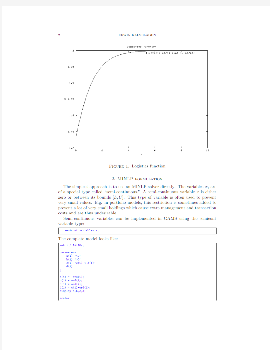
Indeed the functions

(2)f i(x)=c i+

d i?c i

1+exp

?x?a i

b i

are convex,as can be seen from the?gure1.

However,the non-convexity introduced by x being not a continuous variable will cause that this model can not be solved using an NLP solver directly.

Date:April,2003.

1

2ER WIN KAL VELAGEN

Figure1.Logistics function

2.MINLP formulation

The simplest approach is to use an MINLP solver directly.The variables x i are of a special type called“semi-continuous.”A semi-continuous variable x is either zero or between its bounds[L,U].This type of variable is often used to prevent very small values.E.g.in portfolio models,this restriction is sometimes added to prevent a lot of very small holdings which cause extra management and transaction costs and are thus undesirable.

Semi-continuous variables can be implemented in GAMS using the semicont variable type:

semicont variables x;

The complete model looks like:

set i/i1*i10/;

parameters

a(i)’<0’

b(i)’>0’

c(i)’c(i)

d(i)

;

a(i)=-ord(i);

b(i)=ord(i);

c(i)=ord(i);

d(i)=c(i)+ord(i);

display a,b,c,d;

scalar

BRANCH-AND-BOUND METHODS FOR AN MINLP MODEL WITH SEMI-CONTINUOUS V ARIABLES3 budget_avail/10/

minx/0.5/

;

*-------------------------------------------------------------

*MINLP model with semi-continuous variables

*-------------------------------------------------------------

variables

x1(i)

z1

;

semicont variable x1;

equations

logistic1

budget1

;

logistic1..z1=e=sum(i,c(i)+(d(i)-c(i))/(1+exp(-(x1(i)-a(i))/b(i))));

budget1..sum(i,x1(i))=l=budget_avail;

x1.lo(i)=minx;

model m1/logistic1,budget1/

option minlp=sbb;

option optcr=0;

solve m1maximizing z1using minlp;

Semi-continuous variables can be easily converted to a formulation with binary variables.This can be important if the solver does not support semi-continuous variables.The reformulation looks like:

x≤Uy

x≥Ly

(3)

x∈[0,U]

y∈{0,1}

It is needed that a tight upper bound U on x is available.In our case we know that

x i≤B and thus x i≤B.

i

*-------------------------------------------------------------

*MINLP model with binary variables

*-------------------------------------------------------------

variables

x2(i)

y2(i)

z2

;

binary variable y2;

positive variable x2;

equations

logistic2

budget2

bigm2a(i)

bigm2b(i)

;

scalar bigM;

bigM=budget_avail;

logistic2..z2=e=sum(i,c(i)+(d(i)-c(i))/(1+exp(-(x2(i)-a(i))/b(i))));

budget2..sum(i,x2(i))=l=budget_avail;

bigm2a(i)..x2(i)=l=bigM*y2(i);

bigm2b(i)..x2(i)=g=minx*y2(i);

4ER WIN KAL VELAGEN

model m2/logistic2,budget2,bigm2a,bigm2b/

option minlp=sbb;

option optcr=0;

solve m2maximizing z2using minlp;

The convexity will assure that the subproblems of the branch-and-solver SBB[3] can be solved to optimality,and thus that we?nd a global optimum solution.

3.Piecewise linear approximation

The above model can be tackled by a MIP solver using a piecewise linear formu-lation.As the objective function is a separable function,i.e.:

(4)max

i

f i(x i)

we can use a standard interpolation scheme using so-called SOS2variables(special ordered sets of type two).

Suppose we have tabular data for a scalar function y=f(x)for a given interval x∈[x lo,x up].Let’s denote this data by(ˉx k,ˉy k).We introduce variablesλk with:

X=

k λkˉx k

(5)

Y=

k λkˉy k

(6)

k λk=1

(7)

max2adjacentλ’s nonzero

(8)

λk≥0

(9)

x lo≤X≤x up

(10)

Equation(5)is called the reference row.Equation(6)is known as the function row, and equation(7)is the convexity row.

Theλk variables form a Special Order Set of Type2.In a SOS2set only two adjacent variables of the set can assume non-zero values.

SOS2variables can be implemented in GAMS using the SOS2variable type: sos2variables lambda(k);

The exact de?nition of SOS2variables is solver speci?c,especially in special cases where nonzero lower bounds are used.In the above case we have addedλk≥0, which only leaves the“max two adjacentλ’s are nonzero”which is shared by all solvers that have SOS2facilities.

*-------------------------------------------------------------

*MIP model with piecewise linear objective using SOS2variables

*-------------------------------------------------------------

*

*set up grid(simply equidistant,but with logistic function

*it would be better to use wider grid for larger x)

*

set k/k0*k200/;

scalar stepsize;

stepsize=budget_avail/(card(k)-1);

parameter xbar(i,k),ybar(i,k);

xbar(i,k)=(ord(k)-1)*stepsize;

ybar(i,k)=c(i)+(d(i)-c(i))/(1+exp(-(xbar(i,k)-a(i))/b(i)));

BRANCH-AND-BOUND METHODS FOR AN MINLP MODEL WITH SEMI-CONTINUOUS V ARIABLES 5

y x

?ˉy k ?1ˉx k ?1

?ˉy k

ˉx k

?

ˉy k +1ˉx k +1

?ˉy k +2ˉx k +2

4444444444444

44o o o o o o o o o Figure 2.Linear interpolation

sos2variables lambda3(i,k);

semicont variables x3(i);variables z3,y3(i);x3.lo(i)=minx;

x3.up(i)=budget_avail;equations

refrow3(i)funcrow3(i)convexity3(i)budget3obj3;

refrow3(i)..x3(i)=e=sum(k,lambda3(i,k)*xbar(i,k));funcrow3(i)..y3(i)=e=sum(k,lambda3(i,k)*ybar(i,k));convexity3(i)..sum(k,lambda3(i,k))=e=1;budget3..sum(i,x3(i))=l=budget_avail;obj3..z3=e=sum(i,y3(i));model m3/refrow3,funcrow3,convexity3,budget3,obj3/option mip=cplex;option optcr=0;

solve m3maximizing z3using mip;

It is noted that we have set up an equidistant grid.In this case the logistics function is the most “non-linear”at the beginning while it is almost linear for larger values of x .It could be bene?cial to exploit this property,and space out the grid more for larger values of x .

6ER WIN KAL VELAGEN

As we deal with a convex objective,we can actually drop the SOS2variables and consider them to be continuous:

*-------------------------------------------------------------

*MIP model with piecewise linear objective exploiting convexity

*SOS2variables can be relaxed to positive variables.

*-------------------------------------------------------------

positive variables lambda4(i,k);

semicont variables x4(i);

variables z4,y4(i);

x4.lo(i)=minx;

x4.up(i)=budget_avail;

equations

refrow4(i)

funcrow4(i)

convexity4(i)

budget4

obj4

;

refrow4(i)..x4(i)=e=sum(k,lambda4(i,k)*xbar(i,k));

funcrow4(i)..y4(i)=e=sum(k,lambda4(i,k)*ybar(i,k));

convexity4(i)..sum(k,lambda4(i,k))=e=1;

budget4..sum(i,x4(i))=l=budget_avail;

obj4..z4=e=sum(i,y4(i));

model m4/refrow4,funcrow4,convexity4,budget4,obj4/

option mip=cplex;

option optcr=0;

solve m4maximizing z4using mip;

4.A nonlinear branch-and-bound algorithm

The GAMS language is powerful enough to implement reasonable complex al-gorithms.Examples include Lagrangian Relaxation with subgradient optimization [7],Benders Decomposition[5]and Column Generation algorithms[6].

In this section we implement a branch-and-bound algorithm for the above model.

A standard branch-and-bound algorithm for MINLP problems with integer vari-ables can look like[2]:

{Initialization}

LB:=?∞

UB:=∞

Store root node in waiting node list

while waiting node list is not empty do

{Node selection}

Choose a node from the waiting node list

Remove it from the waiting node list

Solve subproblem

if infeasible then

Node is fathomed

else if optimal then

if integer solution then

if obj>LB then

{Better integer solution found}

LB:=obj

BRANCH-AND-BOUND METHODS FOR AN MINLP MODEL WITH SEMI-CONTINUOUS V ARIABLES7 Remove nodes j from list with UB j

end if

else

{Variable selection}

Find variable x k with factional value v

Create node j new with bound x k≤ v

UB j

new :=obj

Store node j new in waiting node list Create node j new with bound x k≥ v

UB j

new :=obj

Store node j new in waiting node list

end if

else

Stop:problem in solving subproblem

end if

UB=max j UB j

end while

The root node is the problem with the integer restrictions relaxed.For more details consult[1,4,8].

When dealing with semi-continuous variables,we need to change just a few

things.A variable x k is considered fractional if0

k .Secondly the bounds

we add to the newly created nodes are x k≤0and x k≥x lo

k

.

*-------------------------------------------------------------

*simple branch and bound algorithm

*-------------------------------------------------------------

variables

x5(i)

z5

;

positive variable x5;

equations

logistic5

budget5

;

logistic5..z5=e=sum(i,c(i)+(d(i)-c(i))/(1+exp(-(x5(i)-a(i))/b(i)))); budget5..sum(i,x5(i))=l=budget_avail;

model m5/logistic5,budget5/

option nlp=conopt;

*---------------------------------------------------------

*datastructure for node pool

*each node has variables x(i)which is either

*still free,or fixed to zero or with a lowerbound

*of minx.

*---------------------------------------------------------

set node’maximum size of the node pool’/node1*node1000/; parameter bound(node)’node n will have an obj<=bound(n)’;

set fixed(node,i)’variables x(i)are fixed to zero in this node’;

set lowerbound(node,i)’variables x(i)>=minx in this node’;

scalar bestfound’lowerbound in B&B tree’/-INF/;

scalar bestpossible’upperbound in B&B tree’/+INF/;

set newnode(node)’new node(singleton)’;

set waiting(node)’waiting node list’;

set current(node)’current node(singleton except exceptions)’;

8ER WIN KAL VELAGEN parameter log(node,*)’logging information’;

scalar done’terminate’/0/; scalar first’controller for loop’;

scalar first2’controller for loop’;

scalar obj’objective of subproblem’;

scalar maxx;

set w(node);

parameter nodenumber(node);

nodenumber(node)=ord(node);

fixed(node,i)=no;

lowerbound(node,i)=no;

set j(i);

alias(n,node);

*

*add root node to the waiting node list

*

waiting(’node1’)=yes;

current(’node1’)=yes;

newnode(’node1’)=yes;

bound(’node1’)=INF;

loop(node$(not done),

*

*node selection

*

bestpossible=smax(waiting(n),bound(n));

current(n)=no;

current(waiting(n))$(bound(n)=bestpossible)=yes;

first=1;

*

*only consider first in set current

*

loop(current$first,

first=0;

log(node,’node’)=nodenumber(current);

log(node,’ub’)=bestpossible;

*

*remove current node from waiting list

*

waiting(current)=no;

*

*clear bounds

*

x5.lo(i)=0;

x5.up(i)=budget_avail;

*

*set appropriate bounds

*

j(i)=lowerbound(current,i);

x5.lo(j)=minx;

j(i)=fixed(current,i);

x5.up(j)=0;

*

*solve subproblem

*

solve m5maximizing z5using nlp;

BRANCH-AND-BOUND METHODS FOR AN MINLP MODEL WITH SEMI-CONTINUOUS V ARIABLES9 *

*check for optimal solution

*

log(node,’solvestat’)=m5.solvestat;

log(node,’modelstat’)=m5.modelstat;

abort$(m5.solvestat<>1)"Solver did not return ok";

if(m5.modelstat=1or m5.modelstat=2,

*

*get objective

*

obj=z5.l;

log(node,’obj’)=obj;

*

*check"integrality"

*

maxx=smax(i,min(x5.l(i),max(minx-x5.l(i),0)));

if(maxx=0,

*

*found a new"integer"solution

*

log(node,’integer’)=1;

if(obj>bestfound,

*

*improved the best found solution

*

log(node,’best’)=1;

bestfound=obj;

*

*remove all waiting nodes with bound

*

w(n)=no;w(waiting)=yes;

waiting(w)$(bound(w)

);

else

*

*"fractional"solution

*

j(i)=no;

j(i)$(min(x5.l(i),max(minx-x5.l(i),0))=maxx)=yes;

first2=1;

loop(j$first2,

first2=0;

*

*create2new nodes

*

newnode(n)=newnode(n-1);

fixed(newnode,i)=fixed(current,i);

lowerbound(newnode,i)=lowerbound(newnode,i);

bound(newnode)=obj;

waiting(newnode)=yes;

fixed(newnode,j)=yes;

newnode(n)=newnode(n-1);

fixed(newnode,i)=fixed(current,i);

lowerbound(newnode,i)=lowerbound(newnode,i);

bound(newnode)=obj;

waiting(newnode)=yes;

10ER WIN KAL VELAGEN

lowerbound(newnode,j)=yes;

);

);

else

*

*if subproblem as infeasible this node is fathomed.

*otherwise it is an error.

*

abort$(m5.modelstat<>4and m5.modelstat<>5)"Solver did not solve subproblem";

);

log(node,’waiting’)=card(waiting);

);

*

*are there new waiting nodes?

*

done$(card(waiting)=0)=1;

*

*display log

*

display log;

);

The log of this algorithm show it?nds an optimal solution very quickly:

----379PARAMETER log logging information

node ub solvestat modelstat obj integer best waiting

node1 1.000+INF 1.000 2.00097.090 2.000

node2 2.00097.090 1.000 2.00097.089 3.000

node3 3.00097.090 1.000 2.00097.085 4.000

node4 4.00097.089 1.000 2.00097.085 1.000 1.000 1.000

node5 5.00097.089 1.000 2.00097.088 1.000 1.000

The complete model can be downloaded from https://www.wendangku.net/doc/c18580723.html,/~erwin/ bb/bb.gms.

References

1. B.Borchers and J.E.Mitchell,An improved branch and bound algorithm for mixed integer

nonlinear programming,Computers and Operations Research21(1994),359–367.

2.Brian Borchers,(MINLP)Branch and Bound Methods,Encyclopedia of Optimization,vol.3,

Kluwer,2001,pp.331–335.

3.GAMS Development Corp.,SBB,https://www.wendangku.net/doc/c18580723.html,/docs/solver/sbb.pdf,April2002.

4.O.K.Gupta and V.Ravindran,Branch and bound experiments in convex nonlinear integer

programming,Management Science31(1985),no.12,1533–1546.

5.Erwin Kalvelagen,Benders decomposition with GAMS,https://www.wendangku.net/doc/c18580723.html,/~erwin/

benders/benders.pdf,December2002.

6.,Column generation with GAMS,https://www.wendangku.net/doc/c18580723.html,/~erwin/colgen/colgen.pdf,

December2002.

7.,Lagrangian relaxation with GAMS,https://www.wendangku.net/doc/c18580723.html,/~erwin/lagrel/lagrange.

pdf,December2002.

11 BRANCH-AND-BOUND METHODS FOR AN MINLP MODEL WITH SEMI-CONTINUOUS V ARIABLES

8.Sven Ley?er,Integrating SQP and branch-and-bound for mixed integer nonlinear programming,

Computational Optimization and Applications18(2001),295–309.

GAMS Development Corp.,Washington DC

E-mail address:erwin@https://www.wendangku.net/doc/c18580723.html,

罗罗推进器

罗罗S4系列喷水推进器完成海试 升级后的喷水推进器在船舶更低航速时可以提高效率和增加推力 罗罗称，该公司已经成功地完成了第一批S4系列喷水推进器海试。这款产品可以提高船舶在更低速航行时的效率。 据介绍，S4系列喷水推进器是为满足高速轮渡公司减速航行要求专门研制的。虽然以前，为绝大多数高速渡轮设计的服务航速都在45节到45节以上，但由于增加了燃油成本，因此渡轮经营者正在寻求在提高渡轮效率的同时有助于优化降低航速和燃油耗的喷水推进器。 S4系列喷水推进器的试验是在最近升级的Tangalooma Jet号渡轮上进行的。该渡轮为一艘在接近澳大利亚沿海布里斯班航行的可载客350名的高速双体渡轮上。试验结果显示，较之以前安装在该渡轮上的喷水推进器可以提高3%的推力。 Kamewa Waterjets公司在该渡轮上安装了2台63S4喷水推进器来代替Kamewa 63SII 喷水推进器。升级的渡轮上安装了一整套更新改造的驱动机构、包括发动机、喷水推进器的性能完全达到了预期的要求。在渡轮整个航速范围的效率都得到了提高，满足了渡轮以30

节航速运行的要求。由于降低了在某一工作负荷时的燃油耗，因此减少了二氧化碳排放，增加了渡轮的使用范围。船上的液压系统还有助于降低漏油风险。试验还证明采用63S4喷水推进器配套的渡轮的噪声和震动更低，因此大大增加乘客的舒适度。 据悉，采用63S4喷水推进器的渡轮每年可以为船东节省约8万澳元燃油成本。 罗罗公司环驱式永磁推进器首次装船 在经过了几年的开发后，直径1.6米、功率800千瓦的船尾永磁隧道推进器已经装上“Olympic Octopus”号三用工作船（AHTS）并投入运行。 罗-罗公司称，该公司已经向挪威奥林匹克航运公司交付了第一台自己新研制的永磁隧道推进器(TT-PM)。该推进器将装在“Olympic Octopus”号三用工作船（AHTS）上。 永磁隧道推进器的设计概念基于环驱式永磁电动机。该永磁电动机驱动中心的螺旋桨。永磁电动机由两个主要部分组成：一个带若干电线圈绕组的定子和一个若干非常强大的永磁铁的转子。通过与转子上的永磁铁的磁场相互作用的定子建立一个旋转磁场，拖动转子旋转的力，提供机械功率。 与传统的隧道推进器相比，永磁隧道推进器与相同尺寸的推进器相比功率输出高25%，但噪声和振动进一步降低，可以在水下不必进干船坞拆卸。 其他优点包括在传统的隧道推进器安装位置给永磁隧道推进器上面直接空出空间，对

喷水推进技术介绍

船舶喷水推进技术介绍 作者: 望春的排骨发布日期: 2006-7-14 查看数: 2404 出自: https://www.wendangku.net/doc/c18580723.html, 船舶喷水推进技术发展ZT 2004年09月20日 1 喷水推进技术发展概况 喷水推进是一种特殊的船舶推进方式,与螺旋桨不同的是它不是利用推进器直接产生推力,而是利用推进泵喷出水流的反作用力推动船舶前进。与螺旋桨/轴系这一传统的推进方式的理论和应用发展相比,喷水推进进展相当缓慢主要是由于理论研究不成熟,有些关键技术没过关。例如低损失无空泡进口管道系统,高效率和大功能转换能力的推进泵,船、机、泵的有机配合,水动力性能极佳的倒航操纵装置等技术没得到解决等。但喷水推进毕竟具有推进效率高、抗空泡性强、附体阻力小、操纵性好、传动轴系简单、保护性能好、运行噪声低、变工况范围广和利于环保等常规螺旋桨不及的优点。 1.1喷水推进的主要技术发展进程 在船舶喷水推进技术诞生的340年历程中,按时间顺序,大致经历了液泵式喷水推进、间歇式喷水推进、底板式喷水推进、尾板式喷水推进和舷外喷水推进5个阶段。从目前在船舶上的应用情况看,尾板式喷水推进已成为喷水推进的首选型式。 喷水推进装置最早是在1661年由英国人图古德和海斯发明的,直到1839年英国人摩里斯·思凡才发明了一种较为成熟的喷水推进装置,1914年吉尔设计出一种底板式喷水推进系统其上带有一组合式倒车机构,1946年芝加哥分麦克·科拉姆研究出世界上第一个喷水推进舷外机，1962年前苏联首先使用了三级轴流泵和二级轴流泵,1968年美国研制了采用单机双吸离心泵的深浸自控水翼艇,1977年肖特公司成功研发了另一种改进的底板式推进装置——泵喷射推进器,20世纪50年代早期哈密尔顿开始研制尾板式喷水推进器,80年代英国、美国、法国在核潜艇上应用了喷水推进的降噪技术,近几年发展的计算机多点控制实现了操纵性的进一步提高。 曾不断受到船东批评的喷水推进器的部件质量、坚固性和耐用性等问题,由于新型复合材料的应用而得到很大改善。过去曾产生问题的不同金属材料间的电气绝缘和有效的接地屏蔽,在一些新型喷水推进器中也已不再成为问题。

喷水推进器流道对船舶阻力性能的影响

收稿日期：2016-07-04 网络出版时间：2017-3-1316:15 基金项目:国家自然科学基金资助项目（51209048，41176074，51409063）；工信部高技术船舶科研资助项目（G014613002）； 哈尔滨工程大学青年骨干教师支持计划资助项目（HEUCFQ1408） 作者简介：钱浩，男，1980年生，高级工程师。研究方向：舰船总体研究与设计。 宋科委（通信作者），男，1991年生，硕士生。研究方向：喷水推进器。 喷水推进器流道对船舶阻力性能的影响 钱浩1，宋科委2，郭春雨2，龚杰2 1中国船舶及海洋工程设计研究院，上海200011 2哈尔滨工程大学船舶工程学院，黑龙江哈尔滨150001 摘 要：［目的］喷水推进船舶的阻力性能与常规船舶有着很大的不同，喷水推进器流道的存在会改变船舶尾 部流场，对船舶阻力性能有着很大的影响。［方法］以FA1型三体船为计算模型，利用CFD 软件STAR-CCM+，将喷水推进器流道看作附体，对比研究安装不同进流角喷水推进器流道前后船舶尾部流场变化。通过对比流道表面压力分布、船体流线的变化，阐述船舶阻力以及阻力成分产生变化的机理。［结果］结果表明：STAR-CCM+可以实现对于船舶阻力性能的预报；喷水推进器进水流道的安装会增大船舶阻力，主要为压差阻力的增大。［结论］对进水流道倾角的优化可以增进喷水推进船舶的阻力性能。关键词：喷水推进器；船舶阻力；数值模拟；流道中图分类号：U661.31+1 文献标志码：A DOI ：10.3969/j.issn.1673-3185.2017.02.003 Influence of waterjet duct on ship 's resistance performance QIAN Hao 1，SONG Kewei 2，GUO Chunyu 2，GONG Jie 2 1Marine Design and Research Institute of China ，Shanghai 200011，China 2School of Shipbuilding Engineering,Harbin Engineering University ，Harbin 150001，China Abstract ：The waterjet duct can change the flow field of the stern,and it has a great influence on the resistance performance of the ship.The resistance performance of marine vehicles driven by waterjets is very different from that of conventional ships,so it is meaningful to study the changes to the resistance performance of the ship.We used the CFD software STAR-CCM +,treated the waterjet duct as the appendage and compared the change of the flow field in the stern after the installation of the waterjet duct at different angles.We described the change mechanism of the ship 's resistance and resistance components by comparing the change in pressure distribution of the waterjet duct 's surface and the flow field around the hull.The results show that STAR-CCM+can realize the prediction of ship resistance performance because the simulation results achieved perfect accuracy,and it is gradually becoming the development direction of the resistance performance prediction of marine vehicles driven by waterjets.The installation of the waterjet duct will increase the resistance of the ship,which is mainly due to the increase of pressure resistance.In addition,the resistance performance of a ship driven by waterjets can be improved by the optimization of the waterjet duct 's angle. Key words ：waterjets ；ship resistance ；numerical simulation ；duct 引用格式：钱浩，宋科委，郭春雨，等.喷水推进器流道对船舶阻力性能的影响［J ］.中国舰船研究，2017，12（2）：22-29. QIAN H ，SONG K W ，GUO C Y ，et al.Influence of waterjet duct on ship 's resistance performance ［J ］.Chinese Journal of Ship Research ，2017，12（2）：22-29.

喷水推进技术发展概况

喷水推进技术发展概况 武器类资料 2009-09-06 18:48 喷水推进是一种特殊的船舶推进方式,与螺旋桨不同的是它不是利用推进器直接产生推力,而是利用推进泵喷出水流的反作用力推动船舶前进。与螺旋桨/轴系这一传统的推进方式的理论和应用发展相比,喷水推进进展相当缓慢主要是由于理论研究不成熟,有些关键技术没过关。例如低损失无空泡进口管道系统,高效率和大功能转换能力的推进泵,船、机、泵的有机配合,水动力性能极佳的倒航操纵装置等技术没得到解决等。但喷水推进毕竟具有推进效率高、抗空泡性强、附体阻力小、操纵性好、传动轴系简单、保护性能好、运行噪声低、变工况范围广和利于环保等常规螺旋桨不及的优点。 1.1喷水推进的主要技术发展进程 在船舶喷水推进技术诞生的340年历程中,按时间顺序,大致经历了液泵式喷水推进、间歇式喷水推进、底板式喷水推进、尾板式喷水推进和舷外喷水推进5个阶段。从目前在船舶上的应用情况看,尾板式 喷水推进已成为喷水推进的首选型式。 喷水推进装置最早是在1661年由英国人图古德和海斯发明的,直到1839年英国人摩里斯·思凡才发明了一种较为成熟的喷水推进装置,1914年吉尔设计出一种底板式喷水推进系统其上带有一组合式倒车机构,1946年芝加哥分麦克·科拉姆研究出世界上第一个喷水推进舷外机，1962年前苏联首先使用了三级轴流泵和二级轴流泵,1968年美国研制了采用单机双吸离心泵的深浸自控水翼艇,1977年肖特公司成功研发了另一种改进的底板式推进装置——泵喷射推进器,20世纪50年代早期哈密尔顿开始研制尾板式喷水推进器,80年代英国、美国、法国在核潜艇上应用了喷水推进的降噪技术,近几年发展的计算机多点控 制实现了操纵性的进一步提高。 曾不断受到船东批评的喷水推进器的部件质量、坚固性和耐用性等问题,由于新型复合材料的应用而得到很大改善。过去曾产生问题的不同金属材料间的电气绝缘和有效的接地屏蔽,在一些新型喷水推进 器中也已不再成为问题。 1.2喷水推进的主要优点 (1)推进效率较高喷水推进的效率主要取决于推进泵效率和喷水推进系统效率。在保证较高的气蚀比转速的情况下,优良的轴流泵和混流泵的效率目前已达到85%~90%;喷水系统的效率在65%~70%左右。 因此总的推进效率可达50%~63%。 (2)抗空泡能力强 螺旋桨在航速较高时很容易产生空泡,尤其在斜轴推进的快艇上,螺旋桨处于周期性的攻角变化和负荷变化中,使得螺旋桨更易产生空泡和空泡剥蚀,严重的可在几个小时内破坏螺旋桨的叶片。尽管亚空泡和超空泡螺旋桨能够提高抗空泡的能力,但均要牺牲较多的效率。而喷水推进舵叶片具有比螺旋桨更大的抗空泡能力,水流基本上是轴向流,流场比较稳定,减少了空泡剥蚀的机会,而且航速越高喷水推进泵所利用 的冲压就越大,而螺旋桨正相反。这就使高性能船多采用喷水推进的原因。 (3)操纵性和动力定位性能优异 喷水推进船艇的操纵不需要改变主机转速,而主要依靠偏折喷水推进泵喷射出后的高速水流来实现舰船的转向和倒航。倒航装置与喷口的相对位置的变化可做到向前向后任意分配流量,因而,在一定的主机转速下,喷水推进船可以做到无级变速、驻航和倒航。借助转向舵的作用,又可使船舶在正航和倒航时均具有极佳的操纵性,甚至原地回转。而且舵始终处于喷口喷出的高速流中,可保持足够的舵效。如果采用双 机双桨,可以实现船舶横移和原地回转。这是螺旋桨推进方式无法做到的。 (4)工作平稳、噪声低 水推进装置的动叶轮在泵壳内均匀流场中工作,消除了引起动叶轮叶片振动的流体脉动力,明显地改善了泵叶片上的压力分布,可推迟空泡的产生,从而减小叶片的振动和噪声。 (5)适应变工况能力强、主机不易过载 喷水推进泵在转速一定的条件下,推进泵的流量随舰船的不同航速变化并不大,喷水推进装置的功率——航速曲线相当平坦,甚至船舶在系泊状态下,主机转速仍可达到额定转速的90%~95%。这是常规定距 桨所不能做到的。 (6)吃水浅、浅水效应小、传动机构简单、保护性能好。 (7)日常维护和保养较为简易。

喷水推进器资料

DOEN WATERJETS PTy LTD 33 Venture Way, Braeside 3195 Victoria, Australia Tel (+613) 9587 3944 Fax: (+613) 9587 3179 inquiries@https://www.wendangku.net/doc/c18580723.html, The DOEN 200 Series range of models can be matched to engines from 400kW to 4000kW. These high performance units are specially designed and built for continuous commercial use and to meet the exacting standards of marine classification societies. They can be installed as single or as multiple jets in fiberglass, aluminium or steel hulls. They can also be supplied as booster jets. The prefabricated duct is manufactured from Aluminium or Steel plate material resulting in an extremely strong and lightweight structure. The duct is supplied ready to weld or bolt in (vessels). Custom designs are possible to optimise vessel performance and to improve installation and machinery interfacing. The 200 Series waterjets is manufactured using only corrosion resistant materials. The impeller, impeller casing and discharge nozzle are manufactured from stainless steel to provide maximum service life in the most arduous operating environment with extreme resistance to erosion, corrosion and cavitation. The balance of the waterjet is manufactured from marine grade aluminium. This combination of materials provides a new and unique alternative to operators at a very competitive price. A CAN BuS based electronic control system provides a fully integrated multi-station waterjet, engine and marine gear control. The system also provides alarm, monitoring, back up and emergency control function. eDOCk multi function electronic joystick for single lever vector control and close quarter docking is available. The DOEN 100 Series range of models can be matched to engines from 100kW to 900kW. These commercially rated units employ the latest in Waterjet Propulsion technology developed over 40years of in field experience, together with our ongoing Research and Development programs. The 100 Series waterjets are constructed from strong, corrosion resistant and corrosion compatible materials. The stainless steel impeller is a one-piece casting, housed in a stainless steel liner. The intake ducting, impeller casing, and discharge nozzle complete the pump housing and are all manufactured from cast aluminum. The steering and reverse ducting is also manufactured from cast aluminum. A modular construction is used for simplicity of assembly and ongoing maintenance. This minimises the need for special tools to remove these components. The 100 Series pump features a single stage axial flow impeller design, optimised to deliver high volume thrust. This provides superior cavitation resistance and enhanced load-carrying ability together with excellent top speed performance. Each model has a comprehensive range of efficient high thrust impellers which when coupled with DOEN’s engineering expertise in waterjet propulsion application and installation, ensures correct selection and matching of waterjet, engine and gearbox combinations. The DOEN 100 Series of waterjets can be installed as single, twin or triple jets in fibreglass, aluminium and steel hulls. They can also be supplied as booster jets. Performance