Spatial spillover effects of transport infrastructure. evidence from Chinese regions

Spatial spillover effects of transport infrastructure:evidence from Chinese regions
Nannan Yu a ,b ,?,Martin de Jong a ,b ,Servaas Storm b ,Jianing Mi a
a Harbin Institute of Technology,West Dazhi Street 92,150001Harbin,China b
Delft University of Technology,Jaffalaan 5,2628BX Delft,The Netherlands
a r t i c l e i n f o Keywords:
Transport infrastructure Spillover effects Economic growth Spatial Durbin Model China
a b s t r a c t
This paper examines the possibility of spatial spillover effects of transport infrastructure in Chinese regions.We estimate the regional spillovers of the transport infrastructure stock by applying a spatial Durbin Model for the time-period 1978–2009,and also three sub-periods,1978–1990,1991–2000and 2001–2009.The results indicate that positive spillovers exist in each period due to the connectivity characteristic of transport infrastructure at the national level.At the regional level,transport infra-structure spillover effects vary considerably over time among China’s four macro-regions:the eastern region enjoyed positive spillovers all the time;the northeastern region had no signi?cant spillover effects in 1978–1990,negative spillovers in 1991–2000,and positive spillovers in 2001–2009;the central region had negative spillovers for the three sub-periods;for the western region,negative spillovers can be observed after the 1990s.The analysis indicates that changes in spillovers among regions are closely associated with the migration of production factors in China during the last decades.
ó2012Elsevier Ltd.All rights reserved.
1.Introduction
Plenty of studies have been conducted on the impact of trans-port infrastructure development on regional economic growth over the last decades,mostly aiming to examine the economic returns of transport investments in order to ?nd a reasonable investment pattern (Aschauer,1989;Munnell,1990;Ozbay et al.,2003;Can-ning and Bennathan,2007).Even though the range of the measured economic growth effects varies widely among studies,the positive relationship between transport investment and economic develop-ment is now commonly accepted (Banister and Berechman,2001;Berechman et al.,2006).However the ?nding that the impact of transport infrastructure at the regional level is generally lower than the results observed at the national level leads some research-ers to conclude that there exist signi?cant spillover effects across regions.Subsequent research has tried to con?rm this (Munnell,1992;Holtz-Eakin,1994;Cohen and Paul,2004;Cantos et al.,2005;Berechman et al.,2006;Ozbay et al.,2007).Attempts have been made to corroborate the claim that the positive bene?ts accruing from these investments derive not only from investments made by individual states,but that there are also positive external-ities from network expenditures made by neighboring states (Lall,2007).That is because some effects induced by transport infra-structure will extend outside the limits of this area,generating spillover effects (Munnell,1992;Boarnet,1995,1996,1998).
Only a few of studies have focused on ascertaining the possible existence of regional spillovers from transport capital,probably be-cause it is dif?cult to ?nd cases of countries in which its territory is divided in regions with substantial political power as the USA and Spain (Cantos et al.,2005).For the case of the USA,on the one hand,Munnell (1992)found that the impacts of highway capital became smaller as the geographic focus narrowed Thus she hypothesized that highway public capital can create positive cross-state spill-overs because of productivity leakages (spillovers),since the trans-port infrastructure has network characteristics.But Holtz-Eakin and Schwartz (1995)rejected this argument after measuring the spillover effects separately.On the other hand,Boarnet (1995,1996)hypothesized that public capital in?uences economic activ-ity Iargely by shifting that activity from one location to another,and sees this claim con?rmed in the case of the US street-and-highway capital.Considering these two arguments,Berechman et al.(2006)investigated the spillovers of transportation at the state,county and municipality levels of the USA respectively,and they concluded that the spillovers exist at the small geographic areas (at the municipality level)but that they cannot be found at the state and county levels.Ozbay et al.(2007)calculated the con-tribution of transport investments to county output using the data from the New York/New Jersey metropolitan area,and their results showed that the spillover effects decreased with distance from the
0966-6923/$-see front matter ó2012Elsevier Ltd.All rights reserved.https://www.wendangku.net/doc/fe5297555.html,/10.1016/j.jtrangeo.2012.10.009
?Corresponding author at:Harbin Institute of Technology,West Dazhi Street 92,150001Harbin,China.Tel.:+447453098837.
E-mail addresses:nyuhit@https://www.wendangku.net/doc/fe5297555.html, (N.Yu),W.M.deJong@tudelft.nl (M.de Jong),S.T.H.Storm@tudelft.nl (S.Storm),mijianing@https://www.wendangku.net/doc/fe5297555.html, (J.Mi).
investment location.For the case of Spain,1the empirical?ndings show the variance:Cantos et al.(2005)con?rmed the existence of very substantial spillovers;álvarez et al.(2006)did not?nd evi-dence of the existence of spillover effects of public infrastructure using a panel data set of the47mainland Spanish provinces;Moreno and Lopez-Bazo(2007)investigated the economic returns to local and transport infrastructure and found negative spillovers across Spanish regions in transport capital investments.This variance of the results is probably because of the difference between studies in the de?nition of public capital and the econometric models. What’s worthy to note is that most empirical studies measure the spillover effects of transport infrastructure restricting attention to the?rst round neighbors for the purpose of a speci?cation that is lin-
ear in the parameters(Boarnet,1996;Berechman et al.,2006;Ozbay et al.,2007;Moreno and Lopez-Bazo,2007).With the development of spatial econometric techniques(Anselin,2001;LeSage and Pace, 2009),some advanced spatial models recently developed have been employed to capture the spatial externalities of infrastructure (including transport infrastructure)(Gomez-Antonio and Fingleton, 2009;Del Bo and Florio,2012).
Due to its huge size,China is disaggregated into many small administrative units—provincial(or municipality)governments,2 which have acquired substantial?nancial power after the Chinese ?scal decentralization,carried out in the early1990s(Zhang et al., 2007).Each local government(provincial level)has the?scal and political power to make decisions on the planning and investment of its transport construction,considering its individual interests. Hence,following?scal decentralization,it is now possible to inves-tigate for China whether regional transport infrastructure invest-ment does have spillover effects–in terms of economic growth–on neighboring regions.In the case of China,only a small number of previous studies provide a separate analysis of spatial spillover endowments of transport infrastructures(Liu et al.,2007;Zhang, 2009;Liu,2010;Hu and Liu,2009).Liu et al.(2007)investigated the spillovers using the panel data for11cities of Zhejiang province and summarized that the highway infrastructure of other contiguous regions had positive spillover effects on local economic growth. Zhang(2009)estimated the spillover effects in the period1993–2004and con?rmed the existence of spillovers at the national level. Liu(2010)examined the contributions of highway and waterway infrastructure for different geographic levels,including both direct effects and externalities and suggested that the Chinese government should take the spatial correlation of investment impacts into con-sideration in its policy making regarding transport investment.Hu and Liu(2009)investigated the external spillover effects of transpor-tation on China’s economic growth based on the spatial models and found the positive spillover with an elasticity of0.06.These studies attempted to verify the existence of spillovers of transport facilities (or several types of transport infrastructure)in China and some of them indeed found empirical evidence of spillovers.However,most of these studies do not estimate spillover effects at the sub-national level,which would be more useful for the public decision making on the planning for large transport projects.This is why we propose this study,in order to obtain more detailed information of regional out-put productivity with respect to transport investment in a spatial framework,?nd changes in(the magnitude of)spillover effects over time,and try to interpret our?ndings in light of the actual situation in China.
Our study aims to test for the presence of regional spillovers of transport capital and to measure their magnitude both in the coun-try as a whole and in speci?c parts of China.Of particular emphasis in this paper is the regional difference in the spatial effects of transport infrastructure on economic growth.The structure of the paper is as follows.The next section gives a brief descriptive analysis of the expansion of the transport infrastructure network and the regional distribution of transport facilities in China.Sec-tion3introduces the methodology and database to quantify spatial spillovers of transport investment in the Chinese regions,and it also presents the results.To improve our understanding of the re-gional differences in spillover,a deeper analysis of the changes in spillover effects of transport infrastructure among Chinese regions will be presented in Section4.The paper ends with conclusions and policy implications.
2.Transport infrastructures in China:an overview
In the past decades,investment in transport infrastructure in China has seen remarkable growth in parallel with its booming economy.After30years of construction,all types of transport infrastructure have seen signi?cant expansion as shown in Table1.
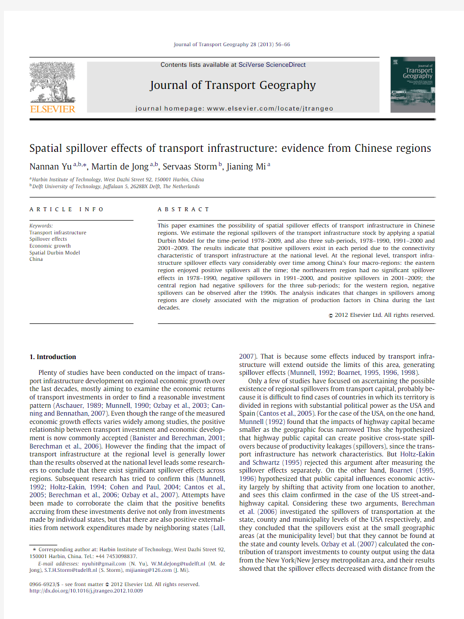
In the past six decades the transport network in China has be-gun to take shape.The patterns of the current railway and highway networks in China in2009are presented in Fig.1.
In2009,the total length of the Chinese railway network reached 103.16thousand kilometers.A government of?cial from the Minis-try of Railways,Mr.Liu Zhijun,3has stated that,in the long-term plan for Chinese railways,the total railway mileages will increase to120thousand kilometers,including16thousand kilometers of high-speed railways in2015.
As to the highways,the investment in the highway construction was as high as RMB623.11billion yuan(about$93billion dollars) in2009and kept a high growth rate from1978,above10%per year.The total mileage of expressways was45thousand kilome-ters in2009,which was an80%increase compared with the length in2002.
The central government allocates its investment budget mostly to those transport facilities,the construction of which is likely to generate high economic returns,such as toll roads,ports and in-ter-city high-speed rail between high-density metropolitan areas. However,because regional Chinese administrative units have their own discretion with respect to the distribution of public invest-ment,local governments make the investment decision in view of their individual economic growth and(often)neglect the(spill-over)impact of their investments on the neighboring areas.As a re-sult,there is considerable underinvestment in the connecting highways(State Roads and Provincial Roads)and rural roads, which have low economic returns but high social returns.
Table1
Transport system mileage in China.Source:The data is obtained from China Transportation Yearbook(1984–2010).
Year Roads
(?1000km)
Railway
(?1000km)
Waterways
(?1000km)
Civil aviation
(?1000km) 195099.6522.273.648.22
1970636.7443.79148.4242.50
1980883.3152.98108.53231.38
19901028.3057.83109.27506.82
20001402.7968.70119.371529.14
20053345.7175.48123.311998.52
20093860.2185.56123.752345.19
1For the case of Spain,several studies on the topic of cross-border spillover effects recently emerged.However,these papers adopted a methodology based on the accessibility calculation in a Geographic Information System support,which was not very related to our paper.Thus,we did not review this literature here.
2The administrative hierarchy in China is:county–city–province(or municipal-
ity)–state.Since the?nancial reform in1994,the provincial(and municipalities) governments have obtained the discretion over priority-setting in public investment.
3Mr.Liu Zhijun was the head of Ministry of Railway Transportation in China during the period of2003–2011,which is independent from the Ministry of Transportation.
N.Yu et al./Journal of Transport Geography28(2013)56–6657
Meanwhile,as we have discussed in our previous paper (Yu et al.,2012),there exists a wide variety in transport infrastructure facilities among Chinese regions 4(shown in Fig.2),which clearly appears as stair steps decreasing gradually from eastern China to western China.Most coastal provinces are well endowed with a high quantity and quality of transport facilities,whereas the transport network density remains very low in remote western provinces.
What is therefore clear is that the transport network has ex-panded considerably since the establishment of modern China in 1949,and because of network characteristics and spatial clustering of transport infrastructures we argue that it is important and nec-essary to consider spatial factors when estimating the potential economic bene?ts of transport facilities.Could the transport facil-ities yield more economic bene?ts than just their direct regional effects on the region alone?How do the spillovers change over time at the sub-national level if the existence of spillovers can be veri?ed?To answer these questions,we will examine the spillover effects at the national and regional level in the next section.3.Measuring spatial spillover effects of transport infrastructure in China
3.1.Model speci?cation and data collection
3.1.1.Model speci?cation
On the subject of impacts with respect to transport infrastruc-ture,most of the previous studies were conducted within the framework of a Cobb–Douglas (C–D)production function (Boarnet,1996,1998;Holtz-Eakin and Schwartz,1995;Hu and Liu,2009;Del Bo and Florio,2012).Therefore,the baseline empirical model is constructed in framework of production function as:
Y ?f eL ;Kc ;Kg ;TI Te1T
where Y denotes output,L denotes labor input,Kc denotes private sector capital stock,Kg represents pubic capital stock (except for
the transport capital stock)and TI stands for the transport infrastructure capital stock.As usual,in the log-linearized reduced version,the estimated parameters can be thought of as GDP elastic-ities to each regressor:
ln Y ?b 0tb 1ln L tb 2ln Kc tb 3ln Kg tb 4ln TI te
e2T
Given that Moran’s I statistic 5suggested that the data were af-fected by spatial autocorrelation,it is necessary for our study to con-sider the role of a change in own and neighboring explanatory and dependent variables by an appropriate spatial econometric model (Anselin,2001).Based on LeSage and Pace (2009),a general spatial model,Spatial Durbin Model (SDM)6could be considered for our empirical analysis:
y ?q Wy tX b th WX ta l n te
e3T
where q is the spatial autocorrelation coef?cient,W is the spatial weight matrix,X is the matrix of control variables (including labor,private capital,public capital and transport infrastructure),l n de-notes an n ?1vector of ones,a ,h and b are vectors of regression coef?cient estimates,and e is the error term.The SDM includes a spatial lag of the dependent variable (Wy )as well as spatial lagged explanatory variables (WX ).An implication of this is that a change in the dependent variable for a single region may affect the depen-dent variable in all other regions by the network effect;meanwhile a change in the explanatory variable for a single observation can potentially affect the dependent variable in all other
observations.
1.China’s railway network (left)and highway network (right)of China in 2009.Source :The information is collected from the of?cial websites of Ministry of Railways Ministry of Transport of China,2010.Available on line:https://www.wendangku.net/doc/fe5297555.html,/,https://www.wendangku.net/doc/fe5297555.html,/.
4
In our paper,China is divided into four macro regions,based on their level of economic development and geographic position:the eastern region,northeastern region,central region and western region.
5
Here we have used the standard Moran’s index (Moran’s I ),as an indicator of spatial autocorrelation.The results of the spatial autocorrelation analysis indicate that there is signi?cant spatial autocorrelation in these models,thus it is necessary to introduce the spatial factors when we calculate the contributions of transport infrastructure on the regional economic growth.The details of calculation process are available from the authors.6
The SDM is a general spatial model,which,in a restricted form,can be interpreted as a spatial autoregressive model (SAR)or spatial error model (SEM).The choice of this unconstrained speci?cation was driven by LM tests and LR tests.Our result shows that the SDM is to be adopted against SAR and SEM.A Hausman test is calculated to select between ?xed and random effects,and the value is -80.95,thus the random effects is more suitable for our spatial panel model at the national level.We also did the calculation process for each small panel,however,we just provide the ?nal results because of the words limitation.But the details are available from the authors.
Combining Eqs.(2)and(3),our key empirical model for the esti-
spillover effects in China can be constructed as:
tb0tb1ln L i;ttb2ln Kc i;ttb3ln Kg i;t
X N j?1w ij ln L j;tth2
X N
j?1
w ij ln Kc j;t
Kg
j;t th4
X N
j?1
w ij ln TI j;tte i;te4T
where Y is real gross domestic product;i and t are the indices of
province and year respectively;j represents nearby provinces
(j–i);w ij is each of the elements in the spatial weights matrix W
that describes the spatial arrangement of the different regions,
and other variables are de?ned as before.In a SDM context,the re-
gional variation in GDP levels is modeled to depend on the GDP lev-
els from the neighboring provinces captured by the spatial lag
vector Wy,as well as the factors input(including L,Kc,Kg and TI)
of neighboring provinces represented by WX.
In this study,a binary contiguity matrix(w bin)is used to con-
struct the spatial weighted matrix(w ij),which assumes only con-
tiguous provinces can in?uence each other:
w ij?
1if the province i has a border with province j
0otherwise
and
P N
j?1
w ij?1.
Here we choose the‘provincial borders’to de?ne the‘spatial
geographic unit’for this study,because they are the containers of
the data we need for our calculations,while the governments in
these units(provinces)surrounded by the provincial borders have
the power to decide on public investments,which is essential for
the policy application of our empirical?ndings.
For w bin,we can get a symmetric spatial matrix of the29Chi-
nese provinces,7as Fig.3shows.
In order to better evaluate spatial spillovers,following LeSage
and Pace(2009),the direct,indirect and total impacts can be calcu-
lated based on the estimators of SDM.These measures capture the
accumulative effect in the Chinese regions of changes in the inde-
pendent variables(including transport infrastructure),which lead
to a change in the long-run steady-state equilibrium.The purpose
was to verify whether the positive effect of an increase in a region’s
transport infrastructure is accompanied by a negative spillover ef-
fect from other regions.What’s worthy to note is that the direct ef-
fect of independent variables is different with the coef?cient b,
Fig.2.Four macro regions in China.
Fig.3.Symmetric spatial matrix of the29Chinese provinces.7We give the explanation of the provinces selection in the data collection part.
since b also contains the feedback effect,representing the effect of the impacts spilling over to the neighboring regions and back to the region itself.
According to LeSage and Pace(2009)and Del Bo and Florio (2012),the SDM speci?cation contains spatially lagged values of both the dependent and the explanatory variables.LeSage and Pace (2009)provided the theoretical framework to interpret these direct and indirect effects,by transforming the spatial weight matrix and by considering the role of off and on diagonal elements.Formally, the SDM can be re-written as:
eI nàq WTy?X btWX htl n atee5Ty?
X k
r?1
S reWTx rtVeWTl n atVeWTee6T
where S reWT?VeWTeI n b rtW h rTand VeWT?eI nàq WTà1.
If we expand Eq.(6)from one region to n regions and transfer to the matrix form,we can get:
y
1
y 2áááy n ?
X k
r?1
S reWT
11
S reWT
12
áááS reWT
1n
S reWT
21
S reWT
22
áááS reWT
2n
............
S reWT
n1
ááááááS reWT
nn
2
66
66
4
3
77
77
5
x1r
x2r
...
x nr
2
66
66
4
3
77
77
5
tVeWTe
e7T
Here,average direct impacts can be obtained as the average of the diagonal elements of matrix S r(W),the average total impacts could be calculated by averaging over all regions the sum of the rows(or columns)of matrix S r(W)and average indirect impacts(spillover ef-fects)were obtained as a difference between the total and direct impacts.Formally:
rTtotal?nà1l0
n S reWT
l n
MerTdirect?nà1treS reWTT
MerTindirect?MerTtotalàMerTdirect
In this way,the sign and magnitude of direct and indirect im-pacts of the explanative variables can be calculated.
Our methodology differs from the previous studies in two ways:?rstly,our model could consider the spillovers from all the regions, not limited to the?rst round neighbors as the previous literatures did(Boarnet,1996;Berechman et al.,2006;Ozbay et al.,2007; Moreno and Lopez-Bazo,2007);secondly,our study uses a more general spatial speci?cation developed recently,both considering the spatial autoregressive model and spatial error model,which could provide a more complete and accurate picture of the spill-over effects than the existed studies(Hu and Liu,2009;Zhang and Yi,2012),especially with respect to transport infrastructure.
To deal with the endogeneity in our model,we apply Maximum Likehood(ML)procedures in estimating spatial panel data models as implemented in the MATLAB.The spatial panel model and the direct and indirect effect can be computed by the spatial econo-metrics library for MATLAB provided by LeSage.Although the Gen-eralized Method of Moments(GMMs)could be regarded as an alternative,GMM usually has to include spatially lagged indepen-dent variables,a requirement that would not allow us to test the in?uence of spatial spillovers(Del Bo and Florio,2012).
3.1.2.Data collection
The data used in this research are collected from a number of different of?cial Chinese sources,including the China Statistical Yearbook(1982–2010),the Statistical Yearbook of Chinese prov-inces,municipalities and PRC’s Statistical Series of60Years(SSB,2010).The spillover effects to sub-national growth in China will be estimated with data of Chinese provincial governments except Hainan province,which is a separate island without any geo-graphic neighbors.The data of Chongqing is combined with those of Sichuan province in this paper,because Chongqing used to be a city in Sichuan province until1997.Some investment data during 1966–1974are unavailable from of?cial sources due to political is-sues during1974–1978,and consequently we use data from a pa-nel of29Chinese provinces for the period1978–2009for which data is available on real GDP,private sector investment,employed population(labor input),transport infrastructure investment and public investment.
The separate investment data in transport infrastructure cannot be found in various sources and we have to adopt the data on ‘‘investment in transport infrastructure and postal service’’from the Statistical Yearbook of provinces and municipalities instead of the transport investment.We calculate the transport infrastruc-ture capital stock,private sector capital stock and public capital stock based on investment data,according to the perpetual inven-tory method(Goldsmith,1951).8
3.2.Results and discussion
In order to compare the changes of the spillover effects over time,we also ran the spillover effects model(Eq.(4))for three sub-periods,1978–1990,1991–2000and2001–2009,respectively. The key results at the national and regional levels are presented in Tables2–4.The spatial autocorrelation coef?cient q is positive and signi?cant in all panels,indicating that the Chinese provinces are characterized by a positive and signi?cant level of spatial correla-tion,with an estimated coef?cient value ranging from0.15to0.39.
3.2.1.Spillover effects at the national level
Table2reports the results of the estimation of the SDM,and we can?nd that the coef?cients of the labor,private capital,public capital and transport infrastructure are positive and signi?cant. In terms of the spatial lagged independent variables,the national output is a positive function of private capital,public capital and transport infrastructure endowment in the neighboring provinces, while the spillover effects of labor is negative,but not signi?cant. This?nding is in line with Zhang and Yi(2012),which concluded that the spillovers of labor in China were mainly limited at the municipality and county level because of its huge distance be-tween areas.
However,these estimators just provide an idea of interactions among provinces,thus we provide the sign and magnitude of the direct and indirect impacts in order to provide the accurate spill-over effects,especially associated with transport infrastructure in Table3.
Our empirical?ndings show that total effects of private capital and public capital variables have positive signs and are signi?cant at the1%level for the entire observation period.Moreover,these two capitals have a similar magnitude of output elasticity(the coef?cients are0.24and0.22),which means that private capital and public capital have almost the same contribution to the output.In our view,this could be because of the fact that after three decades of economic reform,the market factors have played an essential role in the Chinese economy,even though the 8Private sector capital stock was computed using perpetual inventory method as
follows:,where K is the private capital stock in year t;I is the real private investment in?xed assets in constant1978prices;d is the depreciation rate(we assume the depreciation rate of the private capital is9.6%according to Zhang et al.(2004)).The same method was applied to the calculation of other infrastructure capital stock and transport capital stock.The process of the calculation is not provided here due to the word limitation,but available from the authors.
60N.Yu et al./Journal of Transport Geography28(2013)56–66
governments could still partly control the allocation of social re-sources through economic policies.The results also provide a rea-sonable estimate for the labor coef?cient(0.53),which indicates that labor input growth has the largest impact on Chinese real GDP growth;the coef?cient value is very much in line with?nd-ings from earlier studies and growth-accounting analyses for Asia (Zhang,2009;Sahoo et al.,2010).
Considering the impact of transport infrastructure,we?nd that transport infrastructure has a positive total impact on national growth(the coef?cient is0.17),but this impact decreases over time since the direct impact declines during the different periods(the coef?cients are0.26,0.17and0.04in the periods1978–1990, 1991–2000and2001–2009,respectively).The impact of transport infrastructure declines over time,which may be because since the economic reform,investment in transport projects has continu-ously increased,and after some time the marginal returns began to decline.These empirical?ndings are mainly in line with previ-ous studies for the case of China(Zhang,2009;Liu,2010),but pro-viding some difference in the magnitude of elasticities of these inputs since our study has been unfolded in a spatial context, assuming both of the productivity and factor inputs in the neigh-boring provinces could affect the local economy.
For China,as Table3shows,the spillover effect(indirect effect) of transport infrastructure is0.05(the coef?cient is0.05and statis-tically signi?cant),which means transport stock does not only con-tribute to GDP directly but also indirectly through regional spillover effects.This?nding is consistent with Zhang(2009)and Hu and Liu(2009).Meanwhile,we?nd that these spatial spillovers are signi?cantly positive in each period and increase over time:the coef?cients are0.03for the period1978–1990,0.05for1991–2000,and0.08for the years2001–2009,which are statistically different based on a t-test.9
This?nding implies that the spillover effects played a more and more important part in promoting economic growth(the coef?-cients of spillovers increase over time)because of transport net-work expansion.This expansion helps to reduce transportation costs among regions and also brings indirect social externalities due to the improvement of transport network accessibility.The declining transportation cost is propitious to enlarge the domestic market and to facilitate the development of foreign trade,which could stimulate economic growth(Mao and Sheng,2011).
3.2.2.Spillover effects at the regional level
Focusing mainly on the indirect effect of transport infrastruc-ture(represented by l),as can be seen clearly in Table4,the elas-ticities of the spillovers vary considerably among regions in the entire period under study(the coef?cients are0.14,0.04,à0.05 andà0.06for the eastern,northeastern,central and western re-gions,respectively).The neighboring transport investment will lead to positive effects in the eastern region,and the output elastic-ity is very high,0.14,which means the GDP of the eastern region will increase by0.14%if the transport stock in the neighboring re-gion increases by1%.The spillover effect in the northeastern region is also signi?cant and positive(the coef?cient is0.04),but statisti-cally lower than the one of the eastern region.10However,for the
Table2
Estimation results of SDM at the national level.
Variable1978–2009Period1Period2Period3
Constant 1.203(9.23)***0.691(6.92)*** 1.521(14.24)*** 1.304(4.20)*** L0.572(19.89)***0.471(14.39)***0.566(13.52)***0.597(15.58)*** Kc0.141(12.46)***0.069(17.04)***0.100(13.62)***0.148(15.16)*** Kg0.186(13.59)***0.259(13.37)***0.161(13.38)***0.124(12.23)*** TI0.114(16.53)***0.256(15.61)***0.170(15.35)***0.036(5.36)*** q0.231(4.25)***0.307(3.16)***0.279(13.01)***0.264(8.53)*** W?Là0.283(1.65)à0.156(0.31)à0.188(1.37)à0.176(1.32) W?Kc0.073(6.37)***0.046(2.32)**0.061(7.57)***0.082(10.24)*** W?Kg0.022(11.24)***0.002(5.16)***0.030(9.23)***0.047(2.27)** W?TI0.045(7.32)***0.019(12.49)***0.041(7.35)***0.072(13.24)*** Adj.R20.7960.5190.8770.764 Log likelihood177.42153.43164.36148.35
Note:t-statistics are in parentheses.Numbers of observations equals to numbers of years in each period multiplied by29provinces.
?Statistical signi?cance at the10%level.
**Statistical signi?cance at the5%level.
***Statistical signi?cance at the1%level.
Table3
The direct and indirect effects of explanative variables.
Variables1978–2009Period1Period2Period3
Labor Direct effect0.554(23.14)???0.465(14.67)???0.537(6.36)???0.585(26.41)???
Indirect effectà0.123(1.26)à0.114(1.24)à0.144(0.37)à0.140(1.47)
Total0.531(9.45)???0.451(14.43)???0.493(4.75)???0.545(13.28)???
Private capital Direct effect0.149(6.03)???0.074(14.65)???0.103(21.24)???0.154(14.37)???
Indirect effect0.087(15.35)???0.061(9.31)???0.079(4.25)???0.100(6.32)???
Total0.236(21.75)???0.135(4.67)???0.182(10.46)??0.254(13.46)???
Public capital Direct effect0.192(19.24)???0.261(3.65)???0.166(11.46)???0.129(2.23)??
Indirect effect0.031(7.34)???0.003(1.97)??0.037(8.24)???0.054(7.25)???
Total0.223(13.04)???0.264(11.69)???0.203(12.65)???0.183(10.53)???
Transport infrastructure Direct effect0.119(17.21)???0.258(13.46)???0.173(19.47)???0.036(1.99)??
Indirect effect0.054(15.17)???0.027(13.01)???0.051(2.49)??0.084(12.16)???
Total0.173(12.36)???0.285(26.35)???0.224(2.16)??0.120(7.47)???
9The results from the t-test indicate that the elasticities of transport infrastructure
in various periods are statistically different.
10The t-test results verify that the spillovers in the eastern region and the
northeastern region are statistically different.
N.Yu et al./Journal of Transport Geography28(2013)56–6661
central and western regions,the increase of investment in neighbor-ing transport infrastructure may hold back the local economy(the coef?cients have a negative sign).
When we compare our results for the three sub-periods,we can see that the changes in spillovers vary considerably among these regions:
(1)For the eastern region,the transport stock in the neighboring
region has a positive external impact during the whole per-iod.The regression results illustrate that the output elastic-ities of neighboring transport infrastructures for the three sub-periods are signi?cant and positive(the coef?cients are0.06,0.17and0.14).(2)For the northeastern region,no signi?cant spillovers can be
found in period1,but negative spillovers can be observed in the second period(the coef?cient isà0.06).In the last period,positive externalities can be found(the coef?cient is0.03).
(3)In the central region,the estimated coef?cients of spillovers
areà0.02during1978–1990,à0.12during1991–2000,à0.05during2001–2009,which means that the growth of the transport stock in neighboring regions actually had a negative impact on economic growth in the central region all the time.
(4)For the western region,the negative spillovers can be cap-
tured in the last two sub-periods(the coef?cients are
Table4
Estimation results of SDM at the regional level(East,Northeast,Central and West).
Regions Variables1978–2009Period1Period2Period3
Eastern region L0.616(15.61)***0.495(13.12)**0.597(11.90)**0.668(14.32)*** Kc0.167(20.05)***0.092(21.14)***0.150(17.98)***0.283(15.45)***
Kg0.132(16.36)***0.136(10.42)***0.139(18.35)***0.085(19.31)***
TI0.091(2.25)**0.203(2.59)**0.100(2.34)**0.088(0.41)
q0.394(13.54)***0.325(6.47)***0.293(15.35)***0.343(21.35)***
W?Là1.423(1.36)à1.065(1.44)à1.710(0.79)à1.431(1.22)
W?Kc0.101(15.21)***0.093(12.21)***0.064(1.99)*0.125(2.30)**
W?Kg0.031(3.25)***0.023(1.92)*0.021(7.37)***0.035(12.53)***
W?TI0.124(13.56)***0.035(16.34)***0.151(14.74)***0.103(8.42)***
l0.141(16.32)***0.062(6.87)***0.167(7.12)***0.139(14.55)***
Adj.R20.6450.8320.5350.677
Log likelihood149.23136.65104.36157.64
Northeastern region L0.537(12.09)***0.575(16.03)***0.506(2.93)**0.563(10.31)*** Kc0.099(10.02)***0.051(1.98)*0.108(7.61)***0.109(9.05)***
Kg0.179(6.63)***0.214(10.35)***0.166(2.34)**0.173(15.29)***
TI0.141(4.03)***0.221(21.56)***0.193(1.86)*0.110(2.90)**
q0.214(24.68)***0.269(3.74)***0.196(12.71)***0.286(6.74)***
W?Là0.194(0.47)à0.114(2.62)**à0.107(0.74)à0.083(1.29)
W?Kc0.061(14.62)***0.053(1.87)*0.104(0.39)0.086(16.31)***
W?Kg0.056(8.49)***0.046(0.91)0.055(6.74)***0.082(24.26)***
W?TI0.021(12.42)***à0.121(0.64)à0.074(2.36)**0.022(2.50)**
l0.039(9.26)***à0.106(0.47)à0.057(2.14)*0.030(2.79)**
Adj.R20.7830.8320.6630.675
Log likelihood178.57103.24121.01177.36
Central region L0.535(6.36)***0.566(1.86)*0.521(2.03)*0.573(2.74)** Kc0.105(11.20)***0.058(2.33)**0.081(9.71)***0.104(7.89)***
Kg0.169(10.84)***0.181(10.24)***0.200(9.45)***0.143(6.36)***
TI0.194(15.75)***0.171(2.25)**0.163(17.34)***0.209(10.60)***
q0.262(5.32)***0.305(7.15)***0.192(15.26)***0.254(3.86)***
W?Là0.097(1.09)à0.106(0.73)à0.093(1.37)à0.165(1.93)*
W?Kc0.054(16.32)***0.062(6.31)***0.056(14.28)***0.094(14.63)***
W?Kg0.037(6.84)***0.071(1.04)0.102(2.35)**0.089(1.42)
W?TIà0.071(16.42)***à0.033(7.58)***à0.134(1.89)*à0.075(2.61)***
là0.054(8.09)***à0.015(6.23)***à0.122(2.21)**à0.050(2.28)**
Adj.R20.7050.6350.4630.562
Log likelihood132.53144.89161.26105.85
Western region L0.462(14.23)***0.403(32.90)0.345(2.78)**0.387(2.48)** Kc0.126(12.63)***0.080(2.89)**0.061(10.67)***0.133(21.47)***
Kg0.228(13.25)***0.193(15.36)***0.250(2.35)**0.201(12.35)***
TI0.073(13.02)***0.082(2.77)**0.081(2.06)*0.029(0.65)
q0.235(7.47)***0.169(16.73)***0.145(21.63)***0.271(15.36)***
W?Là0.0521(1.36)à0.131(0.14)à0.067(2.20)**à0.133(1.27)
W?Kc0.037(13.63)***0.030(5.62)***0.051(2.36)**0.036(4.74)***
W?Kg0.021(5.17)***0.010(1.98)*0.043(2.04)*0.039(2.59)**
W?TIà0.084(4.25)***à0.107(0.16)à0.135(8.47)***à0.092(2.43)**
là0.061(2.22)**à0.070(0.88)à0.102(10.15)***à0.059(2.44)**
Adj.R20.5470.4950.5370.512
Log likelihood162.54181.26165.52174.27
Note:t-statistics are given in parenthesis.Period1,Period2and Period3represent1978–1990,1990–2000and2001–2009,respectively.Numbers of observations equals to numbers of provinces in each region multiplied by analysis period.Here,we calculated and reported the indirect effect(spillover effects)of transport infrastructure for each region in different periods,represented by l.
*Statistical signi?cance at the10%level.
**Statistical signi?cance at the5%level.
***Statistical signi?cance at the1%level.
62N.Yu et al./Journal of Transport Geography28(2013)56–66
à0.10andà0.06).We do not?nd spillover effects for the ?rst period:according to our estimations,the estimated coef?cients are not statistically signi?cant in period1.
Our empirical?ndings are partly in line with the previous stud-ies(Zhang,2009;Liu,2010;Hu and Liu,2009)at the national level, but show some contradictory results comparing to Liu(2010)at the regional level.That may be because:(1)Our paper adopted an advanced spatial Durbin Model,considering both the spatial lagged dependent and independent variables;meanwhile the spa-tial spillovers from all the regions were measured in our study, which could make our estimators are more accurate and convinc-ing.(2)Only the highway and waterway capital stock have been considered in his paper,while we adopt a broader selection of transport infrastructure data,including railway and aviation investment.We believe the railway constructions have been emphasized by the central government in recent years(several large high speed train projects).Railway networks are supposed to have signi?cant spillover effects.Thus,the incorporation of rail-way investment data may yield changes in the results.(3)The dif-ferent de?nitions of regions may also cause the con?icting results. In order to underline the spatial factors,four macro regions are classi?ed considering the geographic position,instead of the tradi-tional classi?cation(east,central and west regions)according to the economic development level,which would make our estimate results of the spatial spillovers more realistic.
To summarize,the empirical results from this study con?rm the existence of spillover effects of transport infrastructure for the case of China.More speci?cally,changes in the spillovers between Chi-nese regions over time can be observed.For the purpose of an in-depth analysis on the regional difference in spatial spillovers,we will next investigate how the spillovers of transport infrastructure work in China.
4.Analysis on the changes of spillover effects among Chinese regions
Different from the previous studies on the estimation of trans-port spillover effects from a macro view(Zhang,2009;Liu et al., 2007),we analyze the sources of spillovers in this paper:two types of spillover effects can be classi?ed.On the one hand,positive spill-overs can be caused by productivity leakages because of the con-nectivity characteristics of transport facilities(Munnell,1992). On the other hand,spillovers of transport infrastructure may arise from the migration of production factors:mobile factors of produc-tion migrate to places with better transport stock.That migration results in output gains in places with well-developed transport capital stocks and output losses elsewhere,which has been theo-retically veri?ed in previous studies(Boarnet,1996,1998;Moreno and Lopez-Bazo,2007).Thus,in our study,we try to explain the changes in spillover effects by understanding the nature of the spillovers,interpreting our empirical?ndings according to the ac-tual situation in China.
4.1.Spillover effects arising from network characteristics
According to Banister and Berechman(2001),the increase in transport investment in one region could improve the network accessibility of this region and therefore enlarge its market scale. Adam Smith proposed the‘extent of the market’hypothesis:as the size of the market expands,this makes possible a greater divi-sion of labor and hence specialization,and this in turn would allow the economy to expand further and the growth in output and pro-ductivity would cumulate.Krugman(1991)and Fujita et al.(1999) re-formulated Smith’s argument from a viewpoint of external economies of scale and increasing returns to scale.Thus,we can ar-gue that the transport network expansion could stimulate the economy in both the area where the investment happens and the neighboring areas because of the growing market.In other words, the positive network spillover effects could occur when infrastruc-ture investments in one state bene?t people in other states through the transport network(Munnell,1992).
For the case of China,Mao and Sheng(2011)concluded that both economic opening and regional integration have demonstra-bly positive effects on China’s provincial TFP(total factor produc-tivity);Huang and Li(2006)found that the market scale expansion had a positive impact on economic growth adopting the New Economic Geography methodology.So,we can argue that for China,the rapid enlargement of the market scale induced by transport improvement brings many economic bene?ts.Thus,it is reasonable that we?nd the existence of positive spillovers in China at the national level for the entire period under study and for different sub-periods since the transport network could facili-tate the productivity leakages among provinces.However Chinese regions show that transport stock spillovers change over time-periods,probably because of negative spillovers from factor migra-tion,which may counteract positive externalities from market size changes in some sub-state areas.
4.2.Spillover effects arising from mobile factors
Spillovers from factor migration are positive for regions of des-tination,but negative for regions of origin(Boarnet,1996,1998). Changes in inter-regional migration?ows play an essential role in explaining the changes of spillover effects among regions.In the period of1978–1990,the centralized decision-making struc-ture still applied to spatial distribution of the capitals since the economic reform just started,and factor migration was limited. In the second period(1991–2000),China started to implement a market-oriented economy and the exchange of production factors and commodities grew much easier because of lower transport costs and enhanced accessibility.The production factors began to transfer from the poor West,and the intermediate Northeast and Center to the well-developed East.In2000s,the eastern region has witnessed a dramatic development and its productivity over-?ow was expected to bene?t the other regions by the way of indus-trial redistribution.To understand what has happened,we consider how the migration of production factors has changed over time across the four regions in Table5.The table reports the migra-tion of production factors among regions in different periods.
From Table5,we can see the total trend of the net migration va-lue of production factors(capital and labor).Obviously,the central region(the connecting areas)is the victim of those migrations in 1978–2000,when a substantial outward shift of production activ-ities to the eastern region occurred.Remarkably,the northeastern region and western region do not lose as we expected,possibly be-cause of their substantial geographic distance from the well devel-oped eastern region.In the last decade,the production factors have started to shift from the well-developed eastern region to the un-der-developed regions.A large amount of capital shifted to the western region possibly because of the‘Western Development Strategy’started in1999.Since then the central government has invested a lot in the West and also provided favorable policies to attract other outside investments to that region.These?ndings seem totally in line with the actual situation we analyzed before.
4.3.A saldo matrix for the spillover change in different periods
In view of the two sources of spillovers of transport infrastruc-ture,we will construct a balanced matrix to show what happened in Chinese regions.Here,we suppose that transport spillovers
N.Yu et al./Journal of Transport Geography28(2013)56–6663
arising from mobile production factors show the same trend as fac-tor migration,which has been theoretically veri?ed in Moreno and Lopez-Bazo(2007).Meanwhile,we assume that the spillovers hing-ing on the network characteristics of transport facilities are always positive(+)since our empirical?ndings show the autoregressive coef?cient(q)is positive and signi?cant for each case.Conse-quently,we can construct a saldo matrix for the spillover change in different periods in these four regions,as shown in Table6.
In1978–2000,the eastern region has undergone a great capital and labor in?ux,and the spillovers there from factor migration have been positive.Thus,the saldo matrix shows that the two types of effects are of the same sign,which can explain why the spillover effects from the regression?ndings are positive all the time.In period3,our empirical?ndings show that the spillovers lightly decline but remain positive,which con?icts with the saldo matrix(the spillover should be zero).
For the northeastern region,from a balance perspective,the sal-do matrix shows that in period1,the negative spillover accruing from factor migration from the central region to the eastern region counteracted the positive spillover caused by the connectivity characteristic of transport facilities;in period2,the negative spill-over also exceeded the positive one and the saldo remained nega-tive;in period3,these two types of spillover have the same sign (positive),therefore a positive spillover was found.That is because in the last period,the equipment manufacturing industry has con-centrated in the northeastern provinces because of lower transport cost(Liu et al.,2011).These?ndings can help explain the changes in spillover effects with respect to transport infrastructure from our empirical estimate results.
For the central and western regions,the saldo shows the same trend as for the northeastern region.But in the period of2001–2009,our empirical results indicate that negative spillovers exist in the central and western region.However we can see that the sal-do of spillovers should be positive in the last period,which contra-dicts the data.
Indeed,in the last decade,the improvement in the transport network did not result in industrial expansion in the eastern re-gion,which may disappoint some government of?cials who expect that transport infrastructure construction could reduce the gap be-tween regions by realizing the‘industrial gradient transfer’.As the previous literature(Krugman,1991;Fujita et al.,1999;Banister and Berechman,2001)pointed out,in cases where labor migration is limited,the price of labor would increase with the agglomeration of industries(economic activities),and therefore increase the pro-duction cost.Some enterprises may choose to relocate to periphe-ral areas if production costs exceed savings in exchange costs.In this way,the peripheral regions may bene?t from the productivity over?ow from the core region.However in China,the gradual industrial redistribution may not yet have happened because of a seemingly endless supply of cheap manual labor.China has a very substantial rural labor-surplus,about120million persons in2009 (Yi and Ying,2011).Meanwhile,apart from the transport cost and production cost,the economic policies(such as tax policy)played a key part in the industrial redistribution in China.Thus,in the last period,the technology-intensive industries still moved to the east-ern region(Liu et al.,2011)due to agglomeration effects,caused by lower transport costs.The in-migration of economic activities in the last period in the central and western regions(visible in Ta-ble5)occurs because some resource-intensive industries in the eastern region depend on resource exploitation in the central and western regions.Consequently these industries,such as agricul-ture,petroleum and coal extraction,and metal smelting,have to move out of the eastern region into the resource-rich regions in or-der to meet the growing demand of raw materials for the export industries in the last decade(Liu et al.,2011).But this type of industrial redistribution(production factor migration)happened in the central and western regions had nothing to do with trans-port costs.
That is why we can see the positive sign in the last period from our saldo but negative spillovers can be found from our empirical study,in the central and western regions.For the same reason, the economic activities(production factors)migrated from the eastern part in the last period,but it was not because of the trans-port network.The factor migration caused by the transport infra-structure still went into the eastern coastal provinces from the other regions.Thus,it makes sense that we can still?nd positive spillovers in the eastern region over the2001–2009period.
5.Conclusion and policy implications
Much of the evidence on transport infrastructure spillovers has been reported for the states and counties in the developed
Table5
The migration of production factors among regions in various periods.
East Northeast Center West
Capital Labor Trend Capital Labor Trend Capital Labor Trend Capital Labor Trend
Period1+330+391+à39à32àà238à175àà52à78à1978–1990
Period2+7536+2222++à1763à383ààà3735à1331ààà2200à503àà1991–2000
Period3à712à239à+210+68++287+97++455+65+ 2001–2008
Note:‘+’means shift-in and‘à’means shift-out.The data of capital migration are collected from Peng(2008)(unit is RMB one hundred million yuan).The data of labor migration are gathered from Wang et al.(2010)(unit is ten thousand people)and the National Statistical Compilation of Transient population(Ministry of Public Security, 2010).
Table6
Spillover changes of Chinese regions in different periods.
Spillovers East Northeast Center West
Period1Period2Period3Period1Period2Period3Period1Period2Period3Period1Period2Period3
Source1++++++++++++ Source2+++àààà+ààà+ààà+ Saldo+++++00à++0à++0à++
64N.Yu et al./Journal of Transport Geography28(2013)56–66
countries,such as United States and Spain,where there may be no severe lack of infrastructure endowment.Here,in contrast,we pro-vide evidence on the spillover effect of transport stock in the Chi-nese provinces,some of which were characterized by a low level of economic development and also by a short supply of transport infrastructure in most of the periods under analysis.Therefore, some lessons for emerging economies,which are also having a large working population,can be derived from our results.
Based on this study,transport capital is associated with in-creased output within a region,positive network spillovers,and negative(or positive)output spillovers.The positive spillovers ex-ist at the all-China level,but the Chinese regions have considerable variance in their spatial spillovers across the different periods un-der analysis.Economic growth gains from transport infrastructure in the same region may come at the expense of other regions as there is clear evidence of negative spillovers from mobile produc-tion factors.In terms of policy implications,the following conclu-sions are possible.
(1)Based on the empirical results in Sections3.2and4.1,we
suggest that the investment policy should give priority to the development of cross-regional transport networks instead of intra-regional construction.The existence of spa-tial externalities emerging from the contribution of trans-port infrastructure to regional growth implies that the decision for the provision of transport infrastructure should be made within a‘‘supra-regional’’perspective.Due to the network characteristics of transport facilities,the central government should pay special attention to the regional coordination of transport construction among lower admin-istrative units,such as provinces,in order to avoid region-oriented investment modes.By altering investment patterns in transport infrastructure relative to those of the neighbor-ing regions,each region has the ability to modify the size of its transport stock at the expense or to the bene?t of its neighbor(Lall,2007).Thus,the central government should give guidelines and constraints for decision-making by local government on their investment patterns.
(2)According to the analysis in Sections3.2,4.2and4.3,we
believe that at the regional level,relevant industrial policies for the lagging regions are urgently needed due to the exis-tence of negative spillovers.The industrial agglomeration effects induced by transport development will lead to an increased transfer of industrial activity from western,north-eastern,central China to eastern China,especially the tech-nology-intensive industries.Since labor costs have not yet hindered the economic development in the eastern prov-inces,transport infrastructure development cannot generate industrial expansion there.Thus we can deduce that in the coming years,the technology-intensive industries in the other regions would still transfer to the eastern region due to agglomeration effects.Due to the possible presence of negative spillovers of transport infrastructure arising from these factor migrations,local governments in underdevel-oped areas should alter their industrial policies to avoid redistribution of economic activities.Targeted region-spe-ci?c industrial policies are needed,such as favorable tax pol-icies and lower interest rates for loans for investments in local labor-intensive and technology-intensive industries (Liu et al.,2011).
Acknowledgements
We thank the anonymous reviewer and the editor for their con-structive comments and valuable suggestions.We express our appreciation for the support of the project entitled‘Public Policy Simulation Facing Complex Environment’granted National Nature and Science Foundation at China(No.71073037),and Short Term Visiting Study Funding of Harbin Institute of Technology,China. We thank Mr.Yang Yong for his contributions on the map making. References
álvarez,A.,Arias,C.,Orea,L.,2006.Econometric testing of spatial productivity spillovers from public capital.Spanish Treasury178,9–21.
Anselin,L.,2001.Spatial Econometrics:A Companion to Theoretical Econometrics.
Basil Blackwell,Oxford.
Aschauer, D.A.,1989.Is public expenditure productive?Journal of Monetary Economics23(2),177–200.
Banister, D.,Berechman,J.,2001.Transport investment and the promotion of economic growth.Journal of Transport Geography9(3),209–218. Berechman,J.,Ozmen,D.,Ozbay,K.,2006.Empirical analysis of transportation investment and economic development at state,county and municipality levels.
Transportation33(6),537–551.
Boarnet,M.G.,1995.Transportation infrastructure,economic productivity,and geographic scale:aggregate growth versus spatial redistribution.Working Paper No.255.University of California Transportation Center,Berkeley, California.
Boarnet,M.G.,1996.The direct and indirect economic effects of transportation infrastructure.Working Paper No.340,The Transportation Center,University of California,Berkeley,CA.
Boarnet,G.M.,1998.Spillovers and the locational effects of public infrastructure.
Journal of Regional Science38(3),381–400.
Canning,D.,Bennathan,E.,2007.The rate of return to transportation infrastructure.
World Bank Working Paper No.3293.
Cantos,P.,Gumbau-Albert,M.,Maudos,J.,2005.Transport infrastructure,spillover effects and regional growth:evidence of the Spanish case.Transport Reviews25
(1),25–50.
Cohen,J.P.,Paul,C.J.M.,2004.Public infrastructure investment,interstate spatial spillovers,and manufacturing costs.The Review of Economics and Statistics86
(2),551–560.
Del Bo,C.,Florio,M.,2012.Infrastructure and growth in a spatial framework: evidence from the EU regions.European Planning Studies20(8),1393–1414. Fujita,M.,Krugman,P.,Venables,A.J.,1999.The Spatial Economy,Cities,Regions and International Trade.The MIT Press,Cambridge.
Goldsmith,S.B.,1951.A Perpetual Inventory of National Wealth,Studies in Income and Wealth,vol.14.NBER,New York.
Gomez-Antonio,M.,Fingleton,B.,2009.Analysing the impact of public capital stock using the NEG wage equation:a panel data approach.Spatial Economics Research Centre Discussion Paper24.
Holtz-Eakin,D.,1994.Public-sector capital and the productivity puzzle.Review of Economics and Statistics76,12–21.
Holtz-Eakin,D.,Schwartz,E.A.,1995.Spatial productivity spillovers from public infrastructure:evidence from state highways.National Bureau of Economic Research Working Paper No.5004.
Hu,A.,Liu,S.,2009.Transportation,economic growth and spillovers:conclusion based on spatial econometrics.China Industrial Economics5,5–14.
Huang,J.,Li,K.,2006.Export openness,regional market size and economic growth.
Economic Research6,27–38.
Krugman,P.,1991.Increasing returns and economic geography.Journal of Political Economy99,483–499.
Lall,V.S.,2007.Infrastructure and regional growth,growth dynamics and policy relevance for India.The Annals of Regional Science41(3),581–599. LeSage,J.,Pace,R.K.,2009.Introduction to Spatial Econometrics.CRC Press,Boca Raton,FL.
Liu,Y.,2010.Transport infrastructure investment,regional economic growth and the spatial spillover effects-based on highway and marine’s panel data analysis.
China Industrial Economics12,37–46.
Liu,N.,Chen,Y.,Zhou,Q.,2007.Spatial spillover effects of transport infrastructure on regional economic growth.Journal of Southeast University(English Edition) 23,33–39.
Liu,H.,Liu,W.,Liu,Z.,2011.The quantitative study on inter-regional industry transfer.China Industrial Economics9,79–87.
Mao,Q.,Sheng,B.,2011.Economic opening,regional market integration and total factor productivity.China Economic Quarterly11(1),181–210.
Ministry of Public Security,2010.National Statistical Compilation of Transient population.China Statistical Publishing House,Beijing.
Ministry of Transportation,1984–2010.China Transportation Yearbook.China Statistical Publishing House,Beijing.
Moreno,R.,Lopez-Bazo,E.,2007.Returns to local and transport infrastructure under regional spillovers.International Regional Science Review30(1),47–71. Munnell, A.H.,1990.How does public infrastructure affect regional economic performance.New England Economic Review(September–October),11–32. Munnell,A.H.,1992.Policy watch:infrastructure investment and economic growth.
Journal of Economic Perspectives6(4),189–198.
Ozbay,Ozmen-Ertekin, D.,Berechman,J.,2003.Empirical analysis of the relationship between accessibility and economic development.Journal of Urban Planning and Development129(2),97–119.
N.Yu et al./Journal of Transport Geography28(2013)56–6665
Ozbay,K.,Ozmen, D.,Berechman,J.,2007.Contribution of transportation investments to county output.Transport Policy14(4),317–329.
Peng,W.,2008.The in?uence of capital?ow on Chinese three regional economic gap.PhD.Thesis.Fudan University.
Sahoo,P.,Dash,K.R.,Nataraj,G.,2010.Infrastructure development and economic growth in China.Institute of Developing Economies Discussion Paper No.261. State Statistical Bureau(SSB),1982–2010.China Statistical Yearbook.China Statistical Publishing House,Beijing.
State Statistical Bureau,2010.People’s Republic of China’s Statistical Series of60 Years.China Statistical Publishing House,Beijing.
Wang,F.,Guo,S.,Jiang,Q.,https://www.wendangku.net/doc/fe5297555.html,bor migration and regional development in China:a regional CGE analysis.
Yu,N.,de Jong,M.,Storm,S.,Mi,J.,2012.Transport infrastructure,spatial clusters and regional economic growth in China.Transport Reviews32(1),3–28. Zhang,X.,2009.Transport Infrastructure,Spillover,and Regional Economic Growth.
Nanjing University Press,Nanjing.
Zhang,H.,Yi,B.,2012.Infrastructure,spatial spillovers and regional total factor productivity.Economics2,61–67.
Zhang,J.,Wu,G.,Zhang,J.,2004.The estimation of China’s provincial capital stock: 1952-2000.Economic Research10,35–44.
Zhang,J.,Gao,Y.,Fu,Y.,Zhang,H.,2007.Why does China enjoy so much better physical infrastructure?Economic Research4(3),4–19.
66N.Yu et al./Journal of Transport Geography28(2013)56–66
企业环保标语大全
企业环保标语大全 企业环保标语大全 1.保护中发展,发展中保护 2.落实环保责任,完善环保制度 3.环境与人类共存,开发与保护同步 4.垃圾混置是垃圾,垃圾分类是资源 5.建设绿色企业,坚持绿色经营 6.降低生产成本,节约地球资源 7.生产绿色产品,节约地球资源 8.珍惜资源、永续利用 9.依靠科技进步、促进环境保护 10.合理利用资源、保护生态平衡、促进经济持续发展11.保护环境山河美、持续发展事业兴 12.发展经济不能以牺牲环境为代价 13.使用环保材料,减少环境污染 14.推行清洁生产,促进经济社会可持续发展15.推行清洁生产,实现碧水蓝天 16.推行循环经济,提高资源利用水平 17.依靠科技进步,推行清洁生产 18.环境与人类共存,发展与环保同步
19.贯彻环境教育,宣导环保资讯 20.全员参与改善,持续环保社区 21.提高环保意识,争做环保公民 22.让地球远离污染,让绿色走进家园23.有限的资源,无限的循环 24.降低损耗齐用心,开源节流增效益25.节约的是利润,损耗的是财富 26.树立节约意识,倡导节约行为 27.浪费不因量小而为之,节约不因细微而不为28.保护环境降污染,千方百计增效益29.资源节约齐参加,珍惜使用靠大家30.改变观念,废物利用,资源回收,持续发展31.保护环境、就是保护生产力 32.既要金山银山、更要青山绿水 33.提倡绿色生活、实施清洁生产 34.树立节水意识、反对浪费水源 35.提高环境道德水平、建设文明小康城区36.保护环境、造福后代 37.全面建设小康社会、同心共创美好家园38.当环保卫士、做时代公民 39.让大气清新、让天空蔚蓝、让河山碧绿40.企业求发展、环保须先行
(完整版)高中数学新课标学习心得体会
高中数学新课标学习心得体会 通过对新课标的学习,本人有一些心得体会,现汇报如下: 一、课程的基本理念 总体目标中提出的数学知识(包括数学事实、数学活动经验)本人认为可以简单的这样表述:数学知识是“数与形以及演绎”的知识。 1、基本的数学思想 基本数学思想可以概括为三个方面:即“符号与变换的思想”、“集全与对应的思想”和“公理化与结构的思想”,这三者构成了数学思想的最高层次。基于这些基本思想,在具体的教学中要注意渗透,从低年级开始渗透,但不必要进行理论概括。而所谓数学方法则与数学思想互为表里、密切相关,两者都以一定的知识为基础,反过来又促进知识的深化及形成能力。 2、重视数学思维方法 高中数学应注重提高学生的数学思维能力。数学思维的特性:概括性、问题性、相似性。数学思维的结构和形式:结构是一个多因素的动态关联系统,可分成四个方面:数学思维的内容(材料与结果)、基本形式、操作手段(即思维方法)以及个性品质(包括智力与非智力因互素的临控等);其基本形式可分为逻辑思维、形象思维和直觉思维三种类型。 3、应用数学的意识 增强应用数学的意识主要是指在教与学观念转变的前提下,突出主动学习、主动探究。 4、注重信息技术与数学课程的整合 高中数学课程应提倡实现信息技术与课程内容的有机整合,整合的基本原则是有利于学生认识数学的本质。在保证笔算训练的全体细致,尽可能的使用科学型计算器、各种数学教育技术平台,加强数学教学与信息技术的结合,鼓励学生运用计算机、计算器等进行探索和发现。 5、建立合理的科学的评价体系 高中数学课程应建立合理的科学的评价体系,包括评价理念、评价内容、评价形式评价体制等方面。既要关注学生的数学学习的结果,也要关注他们学习的过程;既要关注学生数学学习的水平,也要关注他们在数学活动中表现出来的情感态度的变化,在数学教育中,评价应建立多元化的目标,关注学生个性与潜能的发展。 二、课程设置
大学生毕业晚会主持词
大学生毕业晚会主持词 A:青春是一曲荡气回肠的歌,三年前我们怀着彩色梦想走进了鄂大,三年中我们有过欢笑,流过泪水,经历磨炼,得到成长 B:三年后的今天,我们在这里重温青春过往,因为明天就将各奔天涯。也正因为此,今夜,我们承载了太多的祝福与惦念,寄托了太多的关怀与企盼。 C:今晚,让我们再一次重温,那些感动过我们的人和事:灯火通明的教学楼里用功的身影,篮球场上捍卫集体尊严的男儿霸气,满是欢声笑语的宿舍边不着边际的闲谈…… D:又一个三年轮回之后,在同样微凉的夏夜,你是否会记起校园里的梧桐树,你是否会记起日记本里的书签,那些五彩缤纷的日子? A:无数个三年之后,你们的思念是否会有增无减?在你成长的岁月里,在你闯荡社会的每一天,是否会有那么几个瞬间让你渴望回到过去 B:让我们静静享受一下挑战,在日复一日与时间的赛跑中,你会变得更加坚强,更加神采奕奕!又一个青春之旅从今晚启航,又一个光阴的故事在今晚讲述 C:亲爱的同窗,不要带着离别的愁绪,因为明天又是一个新的起点,因为我们相信再次相逢,我们还是一首动人的歌!D:很高兴今天能有这个机会同大家相聚一堂,共叙离别。就让今天铭刻在我们心间,让母校留住我们的风采! A:今天,我们也非常荣幸的请到了…… B:下面让我们用热烈的掌声有请……上台讲话 结束语A:欢快的舞蹈表达不尽我们对母校的敬意 B:热情的赞歌唱不尽我们对母校的一腔深情
C:流火的六月,我们将带着恩师的叮咛,怀着必胜的信心,走向新的征程 D:绚烂的七月,我们将载着母校的祝愿,带着亲人的希望,向着新的征程扬帆起航A:老师们,同学们,欢送10级毕业生联欢晚会合:到此结束 A李:毕业,是一个沉重的动词; 刘:毕业,是一个让人一生难忘的名词; 李:毕业,是感动时流泪的形容词; 刘:毕业,是当我们以后孤寂时候,带着微笑和遗憾去回想时的副词; 李:毕业,是我们夜半梦醒,触碰不到而无限感伤的虚词。 刘:若干年后,假如我们还能够想起那段时光,也许这不属于难忘,也不属于永远,而仅仅是一段记录了成长经历的回忆。 李:尊敬的各位领导老师 刘:亲爱的各位同学们 合:大家晚上好! 李:很荣幸和大家相聚在这激情如火的六月,在这充满忧伤的六月! 刘:很高兴和大家相聚在“放心去飞,20年后再相聚—毕业晚会”现场! 李:我是李扬 刘:我是刘伟清 李:今天晚会现场非常荣幸的邀请到院系的各位领导和老师们。 刘:让我们首先欢迎…… 李:灿烂的星空曾经铭刻你我的笑容
初中生物第三单元(生物圈中的绿色植物)知识点
第三单元生物圈中的绿色植物 第一章生物圈中有哪些绿色植物 ?1、绿色植物分为四大类群:藻类、苔藓、蕨类、种子植物 一、藻类、苔藓、蕨类植物 ?2、藻类、苔藓、蕨类植物的区别: ?3、藻类,苔藓,蕨类植物的共同点:藻类,苔藓,蕨类植物都不结种子,它们的叶片背面 有孢子囊群,可产生孢子,称为孢子植物,孢子是一种生殖细胞,在温暖潮湿的地方才能萌发和生长,所以说孢子植物的生活离不开水。 4.藻类植物:“春水绿于染” 5.藻类植物既有单细胞,也有多细胞。既有生活在淡水中,也有海水中。 6.多细胞藻类植物整个身体浸没在水中,几乎全身都可以吸收水和无机盐。可以进行光合作用,但没有专门吸收和运输养料以及进行光合作用的器官。 7.藻类植物没有根茎叶的分化。 8.苔藓植物生存在阴湿环境中。有类似根和茎的分化,但是茎中没有导管,叶中没有叶脉,根很简单,称为假根,具有固定作用。 9.苔藓植物可作为监测空气污染程度的指示植物。 10.蕨类植物:有根茎叶的分化,具有输导组织。有些蕨类植物比较高大。 11.蕨类植物用处:①卷柏、贯众可药用②满江红是一种优良绿肥和饲料③蕨类植物遗体层层堆积,经过漫长年代、复杂变化,逐渐变成了煤。 12.藻类植物,苔藓植物,蕨类植物,生殖依靠孢子,所以也被统称为孢子植物。 第二节 二、种子植物 ? 1.、种子的结构 菜豆种子:种皮、胚(胚芽、胚轴、胚根、2片子叶)【双子叶植物,网状叶脉】
玉米种子:果皮和种皮、胚(胚芽、胚轴、胚根、1片子叶)、胚乳【单子叶植物,平行叶脉】种皮:保护里面幼嫩的胚。 胚:新植物体的幼体,由胚芽(发育成茎和叶)、胚轴(发育成连接根和茎的部位)、胚根(发育成根)和子叶组成。胚乳不是胚的结构。 ?2、子叶和胚乳里有营养物质,供给胚发育成幼苗。 ?3、菜豆种子中与子叶相连的结构是胚轴,玉米种子中滴加碘液变蓝的结构是胚乳,说明胚 乳中含有淀粉。 菜豆种子(双子叶植物): 胚轴:发育成根和茎的连接部 胚芽:发育成茎叶芽 胚根:发育成根 子叶(两片):贮存营养物质 种皮:保护 玉米种子(单子叶植物): 果皮和种皮:保护胚 胚乳:贮存营养物质(含有淀粉,遇碘变蓝) 子叶(一片):转运营养物质 胚芽:发育成茎叶芽 胚轴:发育成茎和根的连接部 胚根:发育成根 ?4、菜豆种子和玉米种子的异同 (严格意义来说,一粒玉米就是一个果实) ?5、种子植物比苔藓、蕨类更适应陆地的生活,其中一个重要的原因是能产生种子。 ?6、种子植物包括两大类群:裸子植物和被子植物。 裸子植物:种子裸露着,不能形成果实,常见的裸子植物有松、杉、柏、苏铁、银杏; 被子植物(绿色开花植物):种子外面有果皮包被着,是陆地上分布最广泛的植物类群。(苹果,梨,葡萄,水稻) 第二章被子植物的一生
环保企业文化标语
环保企业文化标语 导读:本文是关于环保企业文化标语,如果觉得很不错,欢迎点评和分享! 1、维护社会公德,保护生态环境。 2、环保时代,健康生活。自由追逐,财富就在咱们手中。 3、引领环保新时尚,创造自由新生活。 4、你环保健康,一起财富自由。 5、改善环境,保护家园;净化环境,美化家园。 6、百业要兴,环保先行。 7、给你“更环保、更健康、更成功”的选择。 8、低碳生活,自由财富。 9、环保新主义,财富由你创,健康自然来! 10、拯救地球,一起动手。 11、人类若不能与其他物种共存,便不能与这个星球共存。 12、做世界一流环保产品,让地球人都身体康健,给财富自由的翅膀。 13、节能环保缔造健康生活,健康生活成就财富自由。 14、环保进万家,财富赢天下。 15、改善环境,创建美好未来是我们共同的愿望。 16、尽环保力量,谋健康财富。 17、蓝天白云,绿水青山;咱们的发奋,自然的美丽。
18、绿色环保,引领时尚。 19、咱们所拥有的不仅仅是财富,还有干净的水滋养身体。 20、一草一木要爱惜,环境生活创佳绩。 21、落实环境职责,完善环保制度。 22、既要金山银山,更要青山绿水。 23、树立企业形象,协调人与自然。 24、我们期待世界更蓝的天空,期待你灿烂的微笑,期待社会自由的财富。 25、悠然一心,财富自由。 26、争做环保使者,共创绿色礼貌。 27、改善生态环境,营造绿色家园。 28、节能为环保,财富又自由。 29、环保创造健康,财富携手自由。 30、我们所拥有的不仅是财富,还有干净的水滋养身体。 31、财富我创造,自由交给你,享受健康,享受绿色,享受美好生活。 32、绿色与生命共存,健康与财富共进。 33、环保又健康,财富享自由。 34、你我环保,一齐健康,共创财富,共享自由。 35、树环保意识,创健康财富。 36、创意节能环保,缔造健康生活,共创幸福财富,分享快乐自由。
乡村小学语文小班化教学策略研究
龙源期刊网 https://www.wendangku.net/doc/fe5297555.html, 乡村小学语文小班化教学策略研究 作者:仇家凤 来源:《文理导航》2020年第06期 【摘要】随着城镇化进程加快,大量农民向城镇转移,农村学生数减少,小班化教学成为现实。本文针对这一背景,就语文小班化教学的策略进行探讨,希望促进小学语文教学效果的提升。 【关键词】乡村小学;小班化教学;教学策略 近年来国内经济的快速发展吸引越来越多的农村劳动力进入城市谋取工作和发展机会。与此同时,农村学校的生源在逐渐减少,造成这种情况的原因一方面是由于国内长期以来施行的计划生育政策,另一方面务工人员将自己的子女带入城市,以此可以让他们享受到城市里良好的教育条件和环境。上述情况从客观上导致农村学校的适龄学生流失率越来越高,原来的大班在容量上逐渐缩减为小班,甚至是几名学生。农村教师在适应了之前的大班授课后,不得不面对目前农村学校这种急剧变化的教育情况,尤其是作为小学教育主课程的语文科目,其教学人员更需要考虑如何及时应对这些变化。 一、树立小班化教学理念 小班化给教育教学带来了新的契机。语文教学中的小班教学在表面上是指在学生数量较少的班级中进行的语文教学活动,而从更深层次的内容上来说,这种语文教学小班化其实是一种教育方式和方法的发展趋势,更是一种教学理念的演进。为了真正实现学生在语文课堂中能够以主体地位来参与到语文教学活动的各个环节,语文教师要在这里充当好教学引导者的角色。要重视学生在教学中的个性化发展,多阅读一些有利于提升语文阅读能力的文章,同时还要去积极探索有益的教学方法和策略,多赋予孩子学习的主动性,以此激发学生在小班化语文教学活动中的想象力和创造力,实现教育对人的引领和改造作用。 二、增强学生学习自信,发掘学生潜能 课堂教学是师生互动最重要的舞台,“在教学互动中提升质量”是关键,“充分挖掘每一个孩子的潜能”是目标。要努力实现这一目标,必须做到充分尊重每个学生的能力差异。抓住学生的闪光点,在同学、家长面前表扬。讲究语言艺术,让学生感受被赏识的快乐,用真诚的微笑和期待的目光面对每一个孩子,帮助学生树立信心。 三、尊重差异,实施“分层教学”
初中生物生物圈中的绿色植物知识点习题及答案
第三专题 生物圈中的绿色植物 一、绿色植物与生物圈的水循环 [知识网络结构] 水就是植物体的重要组成成分 原因 水保持植物直立的姿态,有利于进行光合作用 1、绿色植物的生活需要水 无机盐只有溶解在水中,才能被吸收与运输 水影响植物的分布:降水量大的地方,植被茂密 根吸水的部位:主要就是根尖成熟区, 吸水 成熟区的特点:生有大量根毛,增大根吸水的表面积 2、水分进入植物体内的途径 途径:木质部的导管 水分的运输 方向:自下而上 树皮:韧皮部中有筛管,输导有机物 茎的结构 形成层:细胞能分裂(木本植物有此结构) 木质部:有导管,输导水分与无机盐 实验:观察叶片的结构(练习徒手切片) 表皮(上、下表皮) 叶片的结构 叶肉 叶脉 重要结构:气孔,就是植物蒸腾失水的门户,也就是气体交换的窗口,由成对的保卫细 胞围成,气孔的开闭由保卫细胞控制。当保卫细胞吸水膨胀时,气孔张开, 当保卫细胞失水收缩时,气孔关闭。 概念:水分以气态从植物体内散发到体外的过程。 蒸腾作用 主要部位:叶片 降低了叶表面的温度 意义 促进对水与无机盐的运输 促进对水的吸收 绿色植物促进了生物圈中的水循环 绿色植物参与生物圈的水循环 提高大气湿度,增加降水量 保持水土 [课标考点解读] 绿色植物促进了生物圈中的水循环,因此保护森林与植被有非常重要的意义。本章重点阐明水就是绿色 植物生存的必要条件,水对植被的影响,植物吸水的主要部位及特点,水运输的途径,蒸腾作用的意义。在能力培养方面,通过解读数据,培养学生的探究能力。 [典型例题剖析] 例1、把发蔫的菠菜泡在清水中,菠菜又重新挺起来,这说明( ) A 、水就是光合作用的原料 B 、水就是溶解与运输物质的溶剂 C 、水能保持植物体固有的姿态 D 、水就是植物体重要的组成成分 [解析]:植物体内只有水分充足时,才能保持挺立的姿态,叶片才能舒展,有利于光合作用。本题没有数据说明水就是植物体的重要组成成分,也没有说明水就是如何作为溶剂来溶解无机盐的。本题考察学生对植物需水原因的分析与理解。答案:C 例2、下图所示,植物吸收水分的主要部位就是( ) [解析]:根尖成熟区就是吸水的主要部位,表皮细胞突起,形成大量根毛,大大增加了吸水的面积。本题主要考察学生识图的能力。答案:A 例3、3月12日就是我国的全民植树节,之所以选择这个时候,就是因为( ) A 、正值农闲时节 B 、土壤松散 C 、雨水较多 D 、叶没长出,蒸腾作用很弱 3、绿色植物参与生物圈的水循环
生态环境绿色标杆企业创建方案
市生态环境绿色标杆企业创建 实施方案(试行) 为深入贯彻落实生态环境部《关于加强重污染天气应对夯实应急减排措施的指导意见》和《市打赢蓝天保卫战作战方案暨2018-2020年大气污染防治攻坚行动实施方案》,激励企业积极创建环保绿色标杆,主动减排,制定本方案。 一、总体要求 全面贯彻落实党的十九大精神和绿色发展理念,坚持“污染排放空间换时间”原则,鼓励企业切实承担污染治理主体责任,强化企业自我监管,积极落实各项减排措施。对达到绿色标杆标准的企业,在错峰生产和重污染天气应急(红色应急除外)期间,实行差别化管理,准予不停产、不限产,实现生产经营和污染减排的双赢。 二、实施范围 钢铁、焦化、炭素、陶瓷、玻璃、石灰窑、铸造、炼油与石油化工、制药、农药、涂料、油墨、工业锅炉、页岩砖、木业加工、表面涂装、家具、印刷(限书报刊、本册平板印刷、无VOCs排放的数字印刷)。(其他行业绿色标杆创建标准根据污染治理进程补充制定。) 三、创建要求 (一)基本要求 企业建设和运行有合法手续,上年度亩产效益评级为良好以上、 - 1 -
无重大环境投诉及群体性上访、未发生重大环境事故、没有被国家和省各类督察巡查发现问题并通报、无环境违法排污行为,按要求实现废气污染物排放在线监控,开展自行监测并实现信息公开,有完善的环保管理制度并有专职环保管理人员。 (二)行业创建标准 各行业创建标准见附件1。 四、豁免政策 对于列入错峰生产、重污染应急减排清单企业,达到绿色标杆企业创建标准要求的,在错峰生产、重污染应急(红色除外)期间免予停产、限产(国家和省明确规定必须执行停限产要求的除外)。 五、实施程序 采用企业自愿申报、县区审核、社会公示、市级核发的工作方式,开展生态环境绿色标杆企业认定工作。 (一)企业申报。按照企业自愿参与的原则,由企业向所在县区大气办提交绿色标杆企业申请表(见附件2,纸质版,A4纸打印并装订成册,一式三份)和电子版。 (二)县区审核。各县区大气办依据绿色标杆企业创建标准和豁免政策对申请表进行复核,筛选出符合条件、综合评价较高的绿色标杆企业。 (三)社会公示。对遴选出的绿色标杆企业,各县区大气办在官方网站和主流媒体进行公示,公示时间不少于5个工作日。对公示无异议的企业,报市大气办备案。 - 2 -
小学语文小班化教学案例
小学语文小班化教学案例 -----培养学生自主与合作学习能力的协调发展 一、案例背景 语文课程标准中指出:“倡导自主、合作、探究的学习方式”,由此可见,自主学习与合作探究的学习方式已成为课程改革的目标之一。那么,如何使自主学习与合作探究的学习方式在我们小班化课堂教学中有用地进行呢?通过自己的教学实践,我感到,教师要善于根据学生特点,为他们创设自主与合作学习的条件,才能确实使自主与合作学习落到实处,而不会是“看似课堂上热热闹闹,实则只是摆摆花架子而无实效性”的局面。下面,我就《我为你骄慢》一课的教学作了尝试。《我为你骄慢》是二年级下册一篇叙事性的文章,故事中的小男孩不小心打碎了老奶奶家的玻璃,当时害怕逃跑了,但后来用自己的行动取得老奶奶的原谅,老奶奶为小男孩感到骄慢。教学时,我给他们充分地自读自悟的机会,给他们个性化表达的机会,同时充分利用小班化小组学习的条件,进行组内合作学习,学会讨论、交流。 二、案例描述 1、解放读课文,要求读准字音、读通句子。 2、旁桌互认生字。 3、组长检查词语。 4、想想小男孩和老奶奶之间发生了什么事。根据下面的提示说一说:送报的小男孩,后来。老奶奶为小男孩感到。 (学生从自主学习到组内合作、交流,参与的主动性、积极性很高,学习气氛非常浓重。) 片段二:叙说故事情节; 1、默读课文1、2自然段,然后试着用自己的话向大家介绍“我打碎玻璃”的详尽经过。小组内练说,指名说。 2、引读第三自然段。
说话:我觉得很不自在,是因为。 生1:我觉得很不自在,是因为我打碎了老奶奶家的玻璃,难以为情见老奶奶。 生2:我觉得很不自在,是因为我担心老奶奶知道。 生3:我觉得很不自在,是因为我做了错事,老奶奶却还微笑着对我。 生4:我觉得很不自在,是因为我很后悔逃跑,感到良心不安。 3、默读四、五自然段,说说我是如何向老奶奶道歉的。 提供词语帮助说话: 三个星期过去了攒钱便条信封 xx悄悄地信箱松弛 小组内练说、指名说。 (通过叙说故事情节,让学生将课文的语言有用地迁移于自己的言语实践,这个要求对于中下层次的学生来说有难度,但是先让学生在小组内练习,让小组里会说的同学先说,能为中下层次的同学提供互助学习的机会,形成了一个优良的学习小环境。) 片段三:说话训练; 师:老奶奶为小男孩的什么而骄慢呢? 生1:为他的厚道。 生2:为他的英勇。 师引导:这叫敢于承担责任。 生3:为他的知错就改。 师:当小男孩看到“我为你骄慢”的便条时是什么样的心情?
湘艺版五年级音乐《长白山下的歌谣》教学设计
湘艺版五年级音乐《长白山下的歌谣》 教学设计 《长白山下的歌谣》教学设计 教材版本:湘艺版音乐教材 教学对象:五年级上期 一、教学案例: (一)题:《长白山下的歌谣》音乐综合 (二)教材版本:湘版新标实验教材 (三)年级:五年级 (四)教具准备:钢琴、AI、打击乐器、朝鲜族服饰、长鼓、金达莱花。 (五)教学目标: ①、认知目标:认真听赏朝鲜民歌《道拉基》,学习三拍子节奏特点。 ②、能力目标:通过小组合作学习(设计身势节奏、用长鼓为歌曲伴奏、即兴歌舞等形式)培养学生的创新能力、合作能力,体验朝鲜族民歌的韵律。 ③、情感目标:通过感受性学习歌曲《金达莱花开朵朵红》,了解朝鲜族人民勤劳淳朴、团结互助、热情好客、能歌善舞的优良传统与民族风情。 (六)设计思路: 五十六个民族五十六枝花,生活在吉林省长白山脚下的
朝鲜族,其歌舞有着独特的节奏韵律。湘版新标实验教材五年级上册第八单元题为:《长白山下的歌谣》,它引起了我的研究兴趣。本单元的教育主题为:用民族音乐激发学生的爱国情感,实现多元文化的交流。即:通过音乐去感受民族文化,进而去了解民族文化;反之,通过文化,我们才可以去体验民族音乐,整体地去认识民族音乐。本时选用听赏《桔梗谣》和演唱歌曲《金达莱花开朵朵红》这两部分内容,教学设计的基本思路是:使学生通过多种形式听、唱“长白山下的歌谣”,深刻体验民族音乐“原生态”的美,以及其歌舞文化、思想内涵;在师生平等互动的学习氛围里,通过实践创作、对歌曲的再表现等形式,激发学生热爱民族音乐、热爱我们伟大祖国的情感。 堂教学中我以“新程”为指导思想,对教学设计进行了一些新的尝试。以下结合自己教学实践中的堂教学个案,和大家共同评析与探讨。 (七)教学过程 ᠄ 导入新过程:即“看风景”。 、AI播放《大长今》影片,背景音乐:《大长今》的主题曲《希望》。 (学生起立,跟随老师自由律动。) 师:刚才同学们听到的旋律出自?
初中生物《生物圈中的绿色植物》单元教学设计以及思维导图
初中生物《生物圈中的绿色植物》单元教学设计以及思维导图1 《生物圈中的绿色植物》主题单元教学设计适用年级六年级 所需时间课内共用7课时,每周3课时 主题单元学习概述 本单元是山东科技出版社五四制,生物学六年级下册。本教材改变了以前教材过分强调学科体系完整性的状况,对分类学知识不再详细描述,降低了知识的难度,注重从学 生的生活经验出发,把提高学生的生物科学素养放在首位,重点是植物和生活环境相适应 的特征及在生物圈和人类的关系。 教材的知识编排结构是从生活环境、基本特征、在生物圈中的作用以及与人类的关系等几个方面进行讲述的,既可以对前面生物与环境相互影响的知识进一步巩固和深化, 又可以为后面学习绿色植物对生物圈的重大意义打下基础。本章节安排三节内容,“藻类、苔藓和蕨类植物和种子子植物,”这些植物放在一章内有利于学生对这三类植物的 特征进行横向的比较。 主题单元规划思维导图 主题单元学习目标 知识目标: (1)概述藻类、苔藓和蕨类植物的形态特征与生活环境。(2)了解藻类、苔藓和蕨类植物对生物圈的作用及与人类的关系。(3)知道种子的结构,明白玉米种子和菜豆种子的区别。(4)了解种子植物分为被子植物和裸子植物的依据并能够举例。能力目标: (1)通过对图片的观看、实物的观察,培养和训练观察能力和思维能力。 (2)通过讨论交流和展示,培养团队协作和归纳表达能力。情感态度与价值观: (1)关注生物圈中各种绿色植物及其生存状况,增强同学们的环保意识。 (2)通过展示交流,树立自信自强心。 对应课标:
1.初步具有收集、鉴别和利用课内外的图文资料及其他信息的能力。 2.关注绿色植物的生存状况,形成环保意识。 3.描述细胞分裂的基本过程。 4.描述各类植物的主要特征和生活环境。 5.说出植物在自然界的作用和人类的关系。 主题单元问题设 生物圈中有哪些绿色植物, 计 专题一:藻类植物 (2课时) 专题二:苔藓和蕨类植物 专题划分 (2课时) 专题三:种子植物 (3课时) 专题一专题一藻类植物 所需课时本专题使用2课时 专题一概述 本专题内容在整个单元中起到引导的作用。通过本专题的学习,学生能够知道藻类植物的基本特征和生活环境,明白藻类植物在自然界中的作用及人类对藻类植物的利用。 专题学习目标 知识目标: 概述藻类植物的主要特征和生活环境。 能力目标: 说出藻类植物在自然界中的作用和与人类的关系。 情感态度价值观: 关注藻类植物的生存现状,形成环保意识。
绿色企业行动宣传标语
绿色企业行动宣传标语 标语,绿色企业行动宣传标语 1、绿色发展,有你才有意义,绿色建设,有你才更完美。 2、环保不分民族,生态没有国界。 3、绿色环保构建美好家园,优质服务打造精致企业。 4、碧水蓝天是我家,绿色生产靠大家。 5、青山绿水要靠你我他共同来维护。 6、打造一流绿色企业,为美好生活加油。 7、美丽油田,我是行动者。 8、落实绿色发展,央企责无旁贷。 9、树立水务形象,协调生产与水。 10、绿色企业,绿色家园,绿色企业,绿色中国。 11、做好环保每一处,携手共护水乡缘。 12、山不言,默背负;水不语,静容纳;绿水青山美石化。 13、树立绿色形象,协调生产与水。 14、保护环境光荣,污染环境可耻。 15、少开车,多步走,活到九十九。 16、石化应有自己的色彩。 17、践行绿色发展理念,守护美丽水乡油田。 18、守护水乡油田,奉献绿色能源。 19、绿色科技,人文内涵——中石化,可持续发展的践行者 20、倡低碳减排之风,走持续发展之路。 21、绿化美化净化看石化,靠你靠我靠他靠大家。 22、让我们与绿色同行,让绿色与我们共生。 23、绿色采购绿色供应,转型发展新愿景。 24、做好维护保养,杜绝跑冒滴漏。 25、垃圾分类,达标排放;保护环境,造福人民。 26、坚持企业优化,促进环境保护。
27、与绿色拥抱,生活更美好。 28、回家吧,回到绿色生产的美好。 29、环保是健康之基,绿色是和谐之源 30、坚持水务发展,促进环境保护。 31、用我们的双手,描绘绿色的家园。 32、绿色成就石化。 33、绿色环保低碳行,节能创效做先锋。 34、低碳环保,绿色生产,我们一直在行动。 35、保护石化环境,共建绿色家园。 36、守护蓝天白云,碧水青山,绿色石化等你回家。 37、万绿丛中一点“石化”。 38、汽油柴油,不如绿水长流;春风十里,不如绿色有你。 39、足下留一寸,换来四时春。 40、让中国石化阳光普照,让绿色企业神圣美妙。 41、水乡油田我的家,绿色生产人人夸。 42、绿色石化福社会,青山绿水笑开颜。 43、建优美环境,筑优良业绩,做优秀社管人。 44、让家园更美,让生活更好。 45、绿色发展,科技创新——中石化,带您畅享低碳生活。 46、垃圾分类回收是物有价值,分类投放是人有素质。 47、共建青山绿水,共享幸福安康。 48、聚焦碧水蓝天净土心动,攻关安全环保节能技术。 49、爱的魔力转圈圈,绿色生产让人心花怒放不知疲倦。 50、手牵手维护绿色家园,心连心构筑和谐石化。 51、爱护环境,是我们每一位石油人应尽的责任。 52、发展诚可贵,效益价更高;若为环保故,两者皆可抛。 53、开发资源立足绿色生态,油气稳产呵护碧水蓝天。 54、石化实说:我喜欢绿色。 55、将绿色进行到底,让绿荫遍布天下。
小班化语文教学案例——《清平乐-村居》
小班化语文教学案例——《清平乐村居》 【设计理念】 在课程标准的理念指导下,结合小班化教学的特点,本课的教学设计力求体现:1、师生、生生的互动。2、教学与活动相结合。3、面向全体,异质教学。4、针对个体,同质活动。 【教学内容】 《清平乐村居》是小学语文五年级上册的一篇课文。课文描绘了一幅充满农村生活气息的田园图景。词的上阕长短句相间,而下阕句式整齐,每句韵脚相同,节奏感强。全词描绘了南方一户农家生活劳动的场景:二老融洽,孩子孝顺,老有所养,少有所事,温馨、淳朴,自然。 【学习目标】 1.正确、流利、在感情地朗读课文,在读中感悟田园生活的意境。使学生从中受到美的熏陶;背诵课文。 2.学会本课5个生字。理解由生字组成的词语。 3.初步了解词的有关知识。 4.理解这首词的意思。想象这首词所描绘的情景,并在说的基础上写下来。 【学习小组的建构】 本课的学习小组先采用异质组合的分组法,再采用异质组队的分组法。根据各项语文学习能力(思维能力、朗读能力、书写能力、口语表达能力等)的强弱进行组合。本班共有24人,分为6组,每组4人,分别为1,2,3,4号。把1、2、3、4号同学,在异质组合的分组法中1、2、3、4号同学作为学习伙伴,其中1号为本小组组长,语文阅读,书写等综合能力较强,2号为本小组中相对较弱的同学,3,4号属于中等水平。在异质组队的分组法所有1号的同学座位一组,所有2号的同学也作为一组,所有3号一组,所有4号一组为一组。 【教学过程】 一.导入新课 1.、师:读读我们以前学过的课文,也有一种情趣,我们二年级学过词串: 金秋烟波水乡 芦苇菱藕荷塘 夕阳归舟渔歌 枫叶灯火月光
《新课标下高中数学概念教学的实践与研究》
《新课标下高中数学概念教学的实践与研究》 课题开题报告 浙江温州第二十二中学高洪武325000 一、课题提出的背景及现实意义 新一轮课程改革已经在全国部分省市如火如荼地开展,为了进一步扩大普通高中新课程实验范围,教育部决定从2006年秋季起,福建、浙江、辽宁和安徽4省将全面进入普通高中新课程实验。这将意味着我省教师将真正意义上进入新课程教学的实践与研究了。作为高中数学教师,理所当然将在这一实验过程中扮演着重要的角色。在新课程理念下,对构建数学理论大厦的数学概念如何实施教学是摆在每一位老师面前的一个严峻的课题。 高中数学课程标准指出:数学教学中应加强对基本概念和基本思想的理解和掌握,对一些核心概念和基本思想要贯穿高中数学教学的始终,帮助学生逐步加深理解。长期以来,由于受应试教育的影响,不少数学教师重解题、轻概念造成数学解题与概念脱节、学生对概念含混不清,一知半解,不能很好地理解和运用概念。数学课堂变成了教师进行学生解题技能培训的场所;而学生成了解题的机器,整天机械地按照老师灌输的“程序”进行简单的重复劳作。严重影响了学生思维的发展,能力的提高。这与新课程大力倡导的培养学生探究能力与创新精神已严重背离。那么在新课标下如何才能帮助学生更好、更加深刻地理解数学概念;如何才能灵活地应用数学概念解决数学问题,我想关键的环节还是在于教师如何实施数学概念教学,为此“新课标下高中数学概念教学的实践与研究”课题在这样的背景下应运而生。 二、国内外关于同类课题的研究综述和课题研究的理论依据 1.国内外关于同类课题的研究综述: 国内外关于数学概念教学理论研究是比较多的,对于一些概念课授课方法也是有研究的。但是那些理论的得出和经验的总结都是特定教育环境下的产物;而对于今天所推进的新课程实验(特别是在我国刚刚开始实施阶段),高中数学概念教学理论研究还几乎是一片空白。对于实践研究就更不足为谈了。 2. 课题研究的理论依据: 2-1 一般来说,数学概念要经历感知、理解、保持和应用四种心理过程。数学概念教学主要依据有如下理论: (1)联结理论、媒介理论:联结理论把概念的掌握过程解释为各种特征的重叠过程,尤如用照相机拍摄下来的事物在底片上的重叠,能够冲洗出照片一样。即接受外界刺激然后做出相应的反应。而媒介理论认为内部过程存在一种媒介因素,并用它来解释复杂的人类行动。 (2)同化、顺应理论:皮亚杰认为,概念的掌握过程无非是经历了一个同化与顺应的过程;所谓同化,就是把新概念、新知识接纳入到一个已知的认知结构中去;所谓顺应,就是当原有的认知结构不能纳入新概念时,必须改变已有的认知结构,以适应新概念。 (3)假设理论:假设理论不同于联结理论把概念掌握的过程看成是一个消极被动的过程,并认为学生掌握概念是一个积极制造概念的过程。所谓积极制造概念的过程,就是根据事实进行抽象、推理、概括、提出假设,并将这一假设应用于日后遇到的事例中加以检验的
大学毕业晚会主持词四人
大学毕业晚会主持词四人 四个主持人主持的大学毕业晚会应该怎么说主持词呢下面小编跟大家分享几篇大学毕业晚会主持词,以供参考! 大学毕业晚会主持词一 1.节奏引领时尚,余音环绕广场,新鲜的韵律,高难度的声响,一样为您缔造不一样的完美想象,下面请欣赏来自07音乐班的xxx为您带来的《》相信会给您带来意外的惊喜。 2.铃声清脆鼓铿锵,天山铃舞尽展情,来自天山的自然是蝶飞花影动,美丽各不同,那就让我们停下脚步,一饱眼福,欣赏由xxx为我们带来的舞蹈《天山铃舞》 3. 军中有歌,歌才动情,军旅里飞来一只熟悉的百灵,不错下面就由请xxx为大家献上一首耳熟能详的老歌,《军中飞来一只百灵》 4.炫酷才叫时尚,八零后心之向往,相信大家都一样,需要个性张扬。今天我们特意请来了城市建设学院的武状元优秀团队,为大家献上一段充满活力的XXX,感谢他们的到来,大家掌声欢迎! 5.相信大家都看过一部曾经风靡一时的电影,那是周杰伦曾经推出的一部年度巨献《不能说的秘密》.里面的四手联弹一定给大家留下了不可磨灭的深刻印象,旋律依旧在脑中回响。不过经典一样可以复制,精彩一样能够粘贴,下面给大家带来的这个惊喜,可谓是非常具有特色,一样是所见
不多,机会难得。下面请欣赏xxxx为大家带来的,钢琴四手连弹《军队进行曲》 6.幽幽云水意.漫漫古典情. 诗情画境的晕染为我们带来流动的娴静。请大家随着动人的舞蹈穿越书法的妙境,伴随优雅的琴韵体会超越喧嚣的古韵墨香。下面请欣赏xxx为您带来的xxxx 7.四年的岁月流光见证了你我在辽东学院的欢欣成长,相信由很多即将走出校园的同学都想倾诉衷肠,下面我们就请出来自05对外汉语的毕业生代表xxx听听她如何表达。 8.当你离开的时候,我送走你的只有沉默。当你离开我的时候,我绝不会把泪滴落。这是金达莱花的歌词大意,相信朝鲜族金达莱花的舞姿会像歌词一样优美,让人回味。下面请欣赏xxxx金达莱花。 9.是谁带来远古的呼唤,是谁留下千年的期盼,这首歌自打年初就开始被人重新无数次的翻唱,不过下面的歌曲,同样青藏高原的演唱,绝对会给您用实力带来不一样。由请xxxx 10.因为有爱,我们才牵手,因为有爱,我们才会风雨同舟。与身边爱自己的人共同牵手,一同遨游,幸福生活才能没有尽头。下面欣赏牵手。 11. 我对你的敬仰之情,如滔滔江水,连绵不绝;又如黄河之水,一发不可收拾;相信大家对电影《月光宝盒》中这一
初中生物生物圈中的绿色植物知识点
初中生物生物圈中的绿 色植物知识点 Company number【1089WT-1898YT-1W8CB-9UUT-92108】
第三单元 生物圈中的绿色植物 第一章 生物圈中有哪些绿色植物 1、绿色植物分为四大类群:藻类、苔藓、蕨类、种子植物 一、藻类、苔藓、蕨类植物 2、藻类、苔藓、蕨类植物的区别: 3、藻类,苔藓,蕨类植物的共同点:藻类,苔藓,蕨类植物都不结种子, 它们的叶片背面有孢子囊群,可产生孢子,称为孢子植物,孢子是一种生殖细胞,在温暖潮湿的地方才能萌发和生长,所以说孢子植物的生活离不开水。 4.藻类植物:“春水绿于染” 5.藻类植物既有单细胞,也有多细胞。既有生活在淡水中,也有海水中。 6.多细胞藻类植物整个身体浸没在水中,几乎全身都可以吸收水和无机盐。可以进行光合作用,但没有专门吸收和运输养料以及进行光合作用的器官。 藻类植物 苔藓植物 蕨类植物 生活环境 大多数生活在水中 阴湿陆地上 阴湿陆地上 形态结构特征 没有根、茎、叶的分化 矮小,有茎和叶的分化(茎中无导管,叶中无叶脉),根是假根 有根茎叶的分化,有输导组 织 与人类关 系 释放氧气 监测空气污染的指示植物 遗体形成煤 矿 常见种类 水绵,衣藻,海带等 墙藓,葫芦藓等 肾蕨,满江红等
7.藻类植物没有根茎叶的分化。 8.苔藓植物生存在阴湿环境中。有类似根和茎的分化,但是茎中没有导管,叶中没有叶脉,根很简单,称为假根,具有固定作用。 9.苔藓植物可作为监测空气污染程度的指示植物。 10.蕨类植物:有根茎叶的分化,具有输导组织。有些蕨类植物比较高大。 11.蕨类植物用处:①卷柏、贯众可药用②满江红是一种优良绿肥和饲料③蕨类植物遗体层层堆积,经过漫长年代、复杂变化,逐渐变成了煤。 12.藻类植物,苔藓植物,蕨类植物,生殖依靠孢子,所以也被统称为孢子植物。 第二节 二、种子植物 1.、种子的结构 菜豆种子:种皮、胚(胚芽、胚轴、胚根、2片子叶)【双子叶植物,网状叶脉】 玉米种子:果皮和种皮、胚(胚芽、胚轴、胚根、1片子叶)、胚乳【单子叶植物,平行叶脉】 种皮:保护里面幼嫩的胚。 胚:新植物体的幼体,由胚芽(发育成茎和叶)、胚轴(发育成连接根和茎的部位)、胚根(发育成根)和子叶组成。胚乳不是胚的结构。 2、子叶和胚乳里有营养物质,供给胚发育成幼苗。 3、菜豆种子中与子叶相连的结构是胚轴,玉米种子中滴加碘液变蓝的结构 是胚乳,说明胚乳中含有淀粉。
企业环保标语口号
企业环保标语口号 导读:本文是关于标语大全的文章,如果觉得很不错,欢迎点评和分享! 1、节能为环保,财富为健康。 2、争做环保使者,共创绿色文明。 3、环保创造健康,财富携手自由。 4、支持环保,别让你的健康与财富自由流失。 5、为环保献力,为自己添富。 6、环保进万家,财富赢天下。 7、绿色的,健康的;节能的,世界的。 8、环保障,自然情,人康健,子孙福。 9、以美与人,用善待己。 10、人与自然需要和谐共存。 11、保护生态环境,倡导礼貌新风。 12、践行环保理念,扞卫健康生活。 13、保护环境,保存希望。 14、环保新主义,财富由你创,健康自然来。 15、健康环保,畅享自由财富。 16、青山常在,绿水常流。 17、生态环保,节能先锋,享受生活。 18、共创绿色世界,自由追寻梦想。
19、保护环境,持续发展。 20、这天节约一滴水,留给后人一滴血。 21、守护健康人生,畅享财富自由。 22、产品买环保,处理少烦恼。 23、全面建设小康社会,同心共创完美家园。 24、需求无限,资源有限;善用有限,发展无限。 25、有限的资源,无限的循环。 26、以法保护自然环境,以德建立社会礼貌。 27、环保生活,健康财富。 28、做良心企业,为您的完美生活的保驾护航。 29、改善环境,创建美好未来是我们共同的愿望。 30、欣赏荒野、回归自然。 31、天蓝水清,地绿居佳。 32、心飞翔,身康健,天下一片绿色。 33、与环保同行,与财富共进。 34、用心迎接挑战,实现持续发展。 35、环保畅享绿色人生,健康乐活财富自由。 36、做世界一流环保产品,让地球人都身体康健,给财富自由的翅膀。 37、环保健康手牵手,财富自由心连心。 38、绿色是性命之源,绿色是人类之根。 39、美好的环境来自我们每个人的珍惜和维护。
初中生物绿色植物试题
姓名 __________ 班级 _____________________ 一、选择题 3.春季玉米播种后,接着下了一场大雨,土壤长时间浸水结果玉米出苗很少,其 原因主要是 A. 土壤中养分流失 B. 土壤的派度过低 C. 土壤中水分不足 D. 土壤中空气不足 9. 百色市右江河谷是全国着名的亚热带水果基地、 南菜北运基地和“芒果之乡”, 盛产芒果、荔枝等名优水果。芒果、甜美多汁的芒果肉和芒果种子分别是由花的 哪些结构发育而来的 4.一粒小小的种子能长成参天大树,主要是因为种子中具有 A. 胚芽 B .胚 C.胚乳 7?图1为桃花的结构示意图,图中④ 在受精作用完成后,将发育成 A .种子 B .种皮 C. 果实 D.果皮 9. 农业生产中的施肥,主要为农作物的生长提供 A .有机物 B .水 C.无机盐 D. 氧气 10. 呼吸作用的实质是 A .分解有机物,释放能量 B .合成有机物,释放能量 C.分解有机物,贮存能量 D.合成有机物,贮存能量 11. 自然界中,被称为“天然的碳氧平衡器”的生物是 A .植物 B .动物 C.病毒 D.细菌和真菌 13. 植物体吸收和运输水分的主要结构分别是 A .根毛、导管 B .导管、根毛 C.根毛、根毛 D.导管、导管 14. “芒果、龙眼、荔枝”是百色市右江河谷盛产的名优水果,按植物的类群来分,它们都属于 A.子房、子房壁、胚珠 B. 子房壁、子房、胚珠 C. 子房、胚珠、子房壁 D. 胚珠、子房、子房壁 D.子叶 两 1
A.藻类植物 B.蕨类植物 C.裸子植物 D.被子植物 15. “人间四月芳菲尽,山寺桃花始盛开”。造成这一差异的非生物因素主要是
企业使命标语环保
企业使命标语环保 导读:本文是关于标语大全的文章,如果觉得很不错,欢迎点评和分享! 1、健康又环保,财富自由少不了。 2、开环保新天,辟绿色未来。 3、环保新主义,财富由你创,健康自然来! 4、环保一小步,健康一大步。 5、发展中国环保事业,提高民族健康水平,实现百姓财富自由。 6、美在生态,乐在健康,财富自由,创新追求。 7、环保一份心,享受健康财富生活。 8、健康新节能,绿色自由风。 9、节能环保缔造健康生活,健康生活成就财富自由。 10、绿色环保,造福于民。 11、蓝天白云,绿水青山;我们的努力,自然的美丽。 12、多环保,多健康,更多财富自由。 13、做节能环保小卫士,创自由财富新生活。 14、以环保赢得健康,以品质换来财富自由。 15、领军环保节能行业,共创健康美好生活,享受财富自由明天。 16、争做节能环保企业标杆,缔造健康财富自由生活。
17、绿色节能,创造财富。 18、低碳生活,让你要拥有一切。 19、健康有保障,财富更自由。 20、呼吸洁净空气,享受财富生活。 21、环保生活,健康一生,财富自由,不悔此生。 22、现在做环保,未来当富豪。 23、环保是健康的保证,健康是财富的本钱,财富是自由的天地。 24、节能为环保,财富为健康。 25、悠然一心,财富自由。 26、做节能环保小先锋,享自由财富新生活。 27、健康,环保,财富,三者良性循环。 28、环保创财富,健康奔自由。 29、快乐环保,享受健康,经济自由。 30、做世界一流环保产品,让地球人都身体康健,给财富自由的翅膀。 31、尽环保力量,谋健康财富。 32、践行环保理念,扞卫健康生活。 33、节能就是创造财富,节能就是环保健康。 34、打造中国最优节能环保品牌。 35、更环保,更健康,更自由。 36、环保靠大家,健康你我他,财富和自由就有啦。
小班化小学语文课堂教学模式
小班化小学语文课堂教学模式 凤凰镇何田小学朱建平 小班化教学是建立在素质教育高标准,高要求的教育质量观和现代办学效益观基础上,充分发发挥“小班”本质特征的教学模式。现就有关教学策略方面浅谈几点体会。 一、教学方式的重组 在小班化教学模式中,师生之间的互动关系应得到增强和增加。 1、建立和谐的师生关系。教学是师生间交流沟通的过程,教师要和学生共同分享对教材的理解、课堂给予的快乐。教师的责任就是要成为学生学习的引导者、帮扶者和促进者。教师要转变教育观念,关心学生的心理需求,尊重学生的个性表达,营造一种平等宽容、健康和谐的课堂教学氛围。 2、营造浓郁学习氛围的教室环境。学生是课堂教学的主体,小班化教室环境的布置要以学生为本位,从有利于学生学习成长、有利于教师实施个别化教学去考虑。要把教室布置成为一个学习中心,营造浓郁的书香氛围。如可以在教室内悬挂励志格言、经典名句,张贴学生优秀作品,设立班级小书库,在课桌椅的排列上采取个体独立式或小组组合式,摆放成圆形、方框形、辩论型式、等等,以方便学生开展自学思考、课堂练习和进行一些互动沟通、讨论交流。 3、创设科学的教学情境。教师要注意采取各种方法激发学生强烈的求知欲望,引导学生迅速进入最佳语文学习状态,使他们在兴趣盎然的心理气氛中,跟着教师进入新知识的探索过程中。从教学需要出发,营造或创设与教学内容相适应的场景,力求生动、形象、有趣,以激发他们学习的兴趣,引起学生的情感体验,帮助学生迅速而正确地理解教材内容,促进儿童知识的、能力的、智力的、情感意志的尽可能大的发展。 二、自主探究策略 尊重和落实学生在课堂教学中的主体地位,注重学生在课堂内的自主探究,还学生以学习主动权,让学生有独立认知、思考的过程,是新课改的重要理念之