当前位置：文档库 › 3-D Retinal Layer Segmentation of Macular Optical Coherence Tomography Images with Serous Pigment

3-D Retinal Layer Segmentation of Macular Optical Coherence Tomography Images with Serous Pigment

Abstract—Automated retinal layer segmentation of optical coherence tomography (OCT) images has been successful for normal eyes but becomes challenging for eyes with retinal diseases if the retinal morphology experiences critical changes. We pro-pose a method to automatically segment the retinal layers in 3-D OCT data with serous retinal pigment epithelial detachments (PED), which is a prominent feature of many chorioretinal disease processes. The proposed framework consists of the following steps: fast denoising and B-scan alignment, multi-resolution graph search based surface detection, PED region detection and surface correction above the PED region. The proposed technique was evaluated on a dataset with OCT images from 20 subjects diag-nosed with PED. The experimental results showed that: (1) the overall mean unsigned border positioning error for layer seg-mentation is 7.87±3.36μm, and is comparable to the mean in-ter-observer variability (7.81±2.56 μm). (2) the true positive vo-lume fraction (TPVF), false positive volume fraction (FPVF) and positive predicative value (PPV) for PED volume segmentation are 87.1%, 0.37% and 81.2%, respectively; (3) the average run-ning time is 220s for OCT data of 512×64×480 voxels.

Index Terms—Retinal layer segmentation, pigment epithelium detachment (PED), optical coherence tomography (OCT) Manuscript received July 18, 2014; revised September 10, 2014; accepted September 15, 2014.This work was supported in part by the National Basic Research Program of China (973 Program) under Grant 2014CB748600, and in part by the National Natural Science Foundation of China (NSFC) under Grant 81371629, 6140293, 61401294, 81401451 and 81401472.Asterisk indicates corresponding author.

F. Shi, *X. Chen, H. Zhao, W. Zhu, D. Xiang and E. Gao are with the School of Electronics and Information Engineering, Soochow University, Suzhou, China (email: shifei, xjchen, hmzhao, wfzhu, xiangdehui@https://www.wendangku.net/doc/4817354238.html,, gaoenting@https://www.wendangku.net/doc/4817354238.html,).

M. Sonka is with the Department of Electrical and Computer Engineering, the Department of Radiation Oncology, and the Department of Ophthalmology and Visual Sciences, The University of Iowa, Iowa City, IA 52242 USA (e-mail: milan-sonka@https://www.wendangku.net/doc/4817354238.html,).

H. Chen is with Joint Shantou International Eye Center, Shantou University and the Chinese University of Hong Kong, Shantou, China (email:drchenhaoyu@https://www.wendangku.net/doc/4817354238.html,).

Copyright (c) 2010 IEEE. Personal use of this material is permitted. How-ever, permission to use this material for any other purposes must be obtained from the IEEE by sending a request to pubs-permissions@https://www.wendangku.net/doc/4817354238.html,.

I.I NTRODUCTION

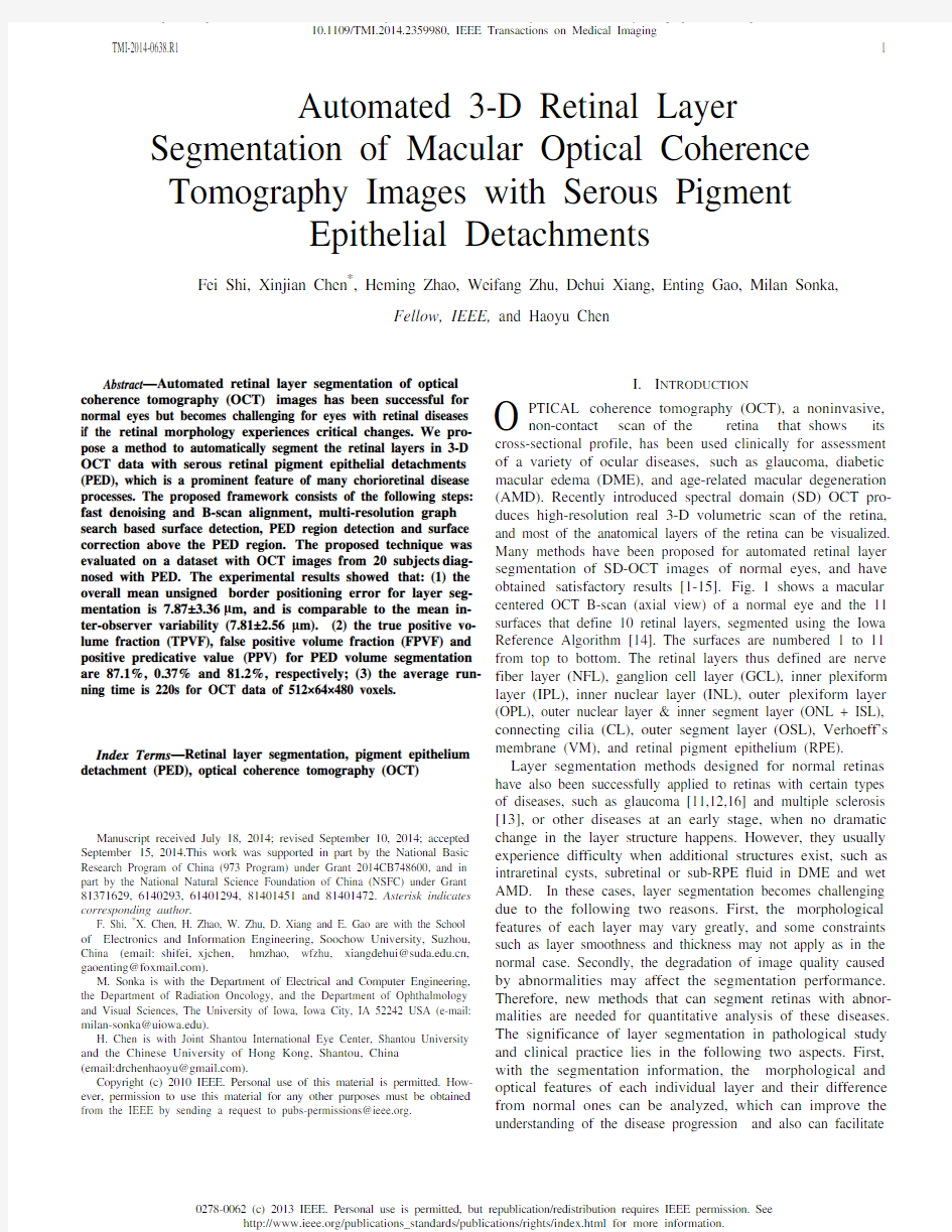
PTICAL coherence tomography (OCT), a noninvasive, non-contact scan of the retina that shows its cross-sectional profile, has been used clinically for assessment of a variety of ocular diseases, such as glaucoma, diabetic macular edema (DME), and age-related macular degeneration (AMD). Recently introduced spectral domain (SD) OCT pro-duces high-resolution real 3-D volumetric scan of the retina, and most of the anatomical layers of the retina can be visualized. Many methods have been proposed for automated retinal layer segmentation of SD-OCT images of normal eyes, and have obtained satisfactory results [1-15]. Fig. 1 shows a macular centered OCT B-scan (axial view) of a normal eye and the 11 surfaces that define 10 retinal layers, segmented using the Iowa Reference Algorithm [14]. The surfaces are numbered 1 to 11 from top to bottom. The retinal layers thus defined are nerve fiber layer (NFL), ganglion cell layer (GCL), inner plexiform layer (IPL), inner nuclear layer (INL), outer plexiform layer (OPL), outer nuclear layer & inner segment layer (ONL + ISL), connecting cilia (CL), outer segment layer (OSL), Verhoeff’s membrane (VM), and retinal pigment epithelium (RPE). Layer segmentation methods designed for normal retinas have also been successfully applied to retinas with certain types of diseases, such as glaucoma [11,12,16] and multiple sclerosis [13], or other diseases at an early stage, when no dramatic change in the layer structure happens. However, they usually experience difficulty when additional structures exist, such as intraretinal cysts, subretinal or sub-RPE fluid in DME and wet AMD. In these cases, layer segmentation becomes challenging due to the following two reasons. First, the morphological features of each layer may vary greatly, and some constraints such as layer smoothness and thickness may not apply as in the normal case. Secondly, the degradation of image quality caused by abnormalities may affect the segmentation performance. Therefore, new methods that can segment retinas with abnor-malities are needed for quantitative analysis of these diseases. The significance of layer segmentation in pathological study and clinical practice lies in the following two aspects. First, with the segmentation information, the morphological and optical features of each individual layer and their difference from normal ones can be analyzed, which can improve the understanding of the disease progression and also can facilitate

Automated 3-D Retinal Layer Segmentation of Macular Optical Coherence Tomography Images with Serous Pigment

Epithelial Detachments

Fei Shi, Xinjian Chen*, Heming Zhao, Weifang Zhu, Dehui Xiang, Enting Gao, Milan Sonka,

Fellow, IEEE, and Haoyu Chen

(a)

(b)

Fig. 1. OCT image of a normal eye and the 11 surfaces defining 10 retinal layers.

(a) B-scan image of OCT volume, obtained using Topcon 3D-OCT 1000. (b) The 11 surfaces overlaid on the OCT image.

diagnosis. Secondly, layer segmentation can localize the ab-normal regions and serve as a pre-processing step for auto-mated detection and analysis of the abnormalities [17-23]. In this paper, we focus on segmentation for retinas with serous pigment epithelium detachments

(PED’s), which is associated with sub-RPE fluid and RPE deformation. We report a fully automated, unsupervised 3-D layer segmentation me-thod for macular-centered OCT images with serous PED’s. In this work, layer segmentation and abnormal region segmenta-tion are effectively integrated, where the position of layers and regions serve as constraints for each other. PED is a prominent feature of many chorioretinal disease processes, including AMD, polypoidal choroidal vasculopathy, central serous chorioretinopathy, and uveitis [24, 25]. PED’s can be classified as serous, fibrovascular, or drusenoid. Study shows that patients diagnosed with serous PED associated with

AMD frequently have co-existing choroidal neovascularization (CNV), or have a higher risk of developing CNV, which can

eventually cause severe visual acuity loss [25, 26]. PED is routinely diagnosed by 2-D imaging techniques such as fluo-rescein angiography (FA) and indocyanine green angiography (ICGV). More recently, SD-OCT offers a means to show the cross-sectional morphologic characteristics of PED and to provide more detailed anatomic assessment. In OCT images, the RPE appears as a bright layer, and serous PED appears as a localized, relatively pronounced dome-shaped elevation of the RPE layer, as shown in Fig.2.

There were several reported methods related to segmentation of OCT images with PED’s or other abnormalities. Penha et al.

Fig. 2. An OCT B-scan showing PED. The red arrow indicates the elevated RPE and the yellow arrow indicates the detached region.

[17] utilized the software on the commercially available Cirrus SD-OCT to detect the RPE and a method proposed by Gregori

et al. [18] to create a virtual RPE floor free of any deformations. The combination of these algorithms permitted the detection of PED’s. The same algorithm was also used to study drusen associated with AMD [18]. Ding et al. [19] detected the top and bottom surfaces of the retina as constraints for subretinal and sub-RPE fluid detection. Chen et al. [20] segmented the flu-id-associated abnormalities associated with AMD using a combined graph-search -graph-cut (GS-GC) method. The ab-normal region was detected together with two auxiliary sur-faces. Dufour et al. [21] detected six surfaces using graph-search based method with soft constraints [7] in OCT images with drusen. Quellec et al. [22] segmented eleven sur-faces in OCT images with fluid-associated abnormalities.

However, all these works focused on region segmentation only. In [17-20], only two or three surfaces were detected and served as constraints for the region segmentation purpose. In [21, 22], more surfaces were detected and their position information was utilized to indicate or detect retinal abnormalities. For all works reported in [17-22], no evaluation of layer segmentation accu-racy was given. In comparison with the existing methods, the proposed me-thod achieves the following goals:

? The retinal OCT image with PED’s is segmented into all discernible layers.

? Both layer segmentation and abnormal region segmentation are performed and high accuracy is achieved.

? The method is designed for retinas with serous PED’s, but it also maintains good performance for normal retinas. II. M ETHOD A. Method Overview

The proposed method consists of pre-processing, layer segmentation and region segmentation (Fig.3). In pre-processing, the OCT scans are first denoised using fast bilateral filtering. Then the B-scans are aligned to correct dis-tortion caused by the eye movement. During layer segmenta-tion, a multi-resolution graph-search method [3, 16] is utilized. Surfaces 1-6 are first detected. Then the elevated RPE floor (surface 11) and the estimated normal RPE floor (defined as surface 12) are detected using the same cost function but dif-ferent smoothness constraints. The positions of surfaces 11 and 12 are used in region segmentation, where their z-axis dis-tance-based difference is used to form a PED footprint map.

Fig. 3. Flowchart of the proposed algorithm

The 3-D PED region is also obtained. Finally, surfaces 7 and

below are detected on a flattened OCT image and are corrected using the PED footprints.

The contribution of this work includes the following:

? A simple and effective alignment method is proposed that improves the performance of the 3-D graph search method while maintaining the natural curvature of retinal layers. ? The normal RPE floor, which does not exist under the PED region, is estimated using 3-D graph search method with simple constraints.

? Layers that are most dramatically affected by PED’s are detected on the flattened image, where their position errors caused by intensity discontinuity can be corrected using geometric constraints. B. Multi-resolution graph search

The 3-D graph search algorithm for optimal surface seg-mentation proposed by Li et al. [27] and its variations were successfully applied to retinal layer segmentation [1-3, 6, 7]. Boundaries between retinal layers can be modeled as ter-rain-like surfaces. Finding the optimal surface is transformed into computing a minimum weight closed set in a node-weighed digraph, which can be solved in polynomial time by computing a minimum s-t cut in a derived arc-weighted digraph [28-30].

Graph search for single surface detection is used in the proposed method. The volumetric image is defined as a 3-D matrix ),,(z y x I with size Z Y X ××, and the surface is de-fined by a function ),(y x S , where }1,,0{?∈X x , }1,,0{?∈Y y , and }1,,0{),(?∈Z y x S . Two parameters, Δx and Δy , control the smoothness of feasible surfaces. More precisely, Δx defines the maximum of )

,(),1(y x S y x S ?+

and Δy defines the maximum of ),()1,(y x S y x S ?+. A cost

function ),,(z y x c inversely related to the likelihood that the voxel belongs to the detected surface is assigned to each voxel, so that the optimal surface is the one with the minimum cost. A node-weighed directed graph ),(E V G is constructed from the volumetric image. Each node in V corresponds to one and only one voxel in ),,(z y x I . The weight of each node is com-puted as

,)1,,(),,(0),,(),,(

??==otherwise z y x c z y x c z if z y x c z y x w (1) so that searching for the optimal surface is transformed to seeking a minimum weight closed set. The arc set E consists of intra-column arcs and inter-column arcs. The intra-column arcs connect each node with its immediate neighbor below, and the inter-column arcs are constructed according to the smoothness constraints, as shown in Fig. 4. This graph is further trans-formed to an arc-weighted digraph where the optimal closed set is found by computing a minimum s-t cut. Refer to [27] for more details.

Two types of cost functions are used in the proposed method. For most layers, the basic edge-based cost function is used. By definition, surfaces 1, 3, 5, 7, 9 and 10 have the dark-to-bright transition from top to bottom of the OCT scan, while surfaces 2, 4, 6, 8 and 11 have the bright-to-dark transition. The Sobel operator is used to calculate the gradient magnitude in z-direction that forms the basic cost function. In the experi-ments, because the test data has low resolution in y-direction, the Sobel operator is calculated in 2-D for each B-scan (x-z plane). An additional region-based cost is calculated and added to the basic edge-based cost for detection of surface 1, to ensure that surface 1 is favored than surface 7, which also has a high-contrast dark-to-bright transition. This cost is a summa-tion of voxel intensities in a limited region above each voxel [1]. Since the region above surface 1 is darker than that above sur-face 7, the voxels on surface 1 can have lower costs than those on surface 7.

Two facts are considered in determining the smoothness constraints Δx and Δy for each surface: the image resolution and the shape of surfaces. If the resolution is high, small values are used to ensure the smoothness of the surfaces. However, when the resolution is low, for certain surfaces, big difference of surface positions may exist between adjacent slices. For

example, surface 1 around the fovea and surface 11 above the PED region may have these quick changes. Therefore, for detection of these surfaces, large values of constraints are needed to ensure feasible surfaces exist. However, with large smoothness constraints, the detected surface position is more easily affected by noise or other artifacts in the OCT scan. The multi-resolution graph search method [3] is used in our algorithm to improve the efficiency of surface detection. The 3-D OCT scan is downsampled by a factor of 2 twice in

z-direction to form three resolution levels. Level 1 represents the lowest resolution and level 3 represents the highest resolu-tion, i.e., the original data. The search for the surface in higher resolution is constrained in a subimage near the position of the surface detected in the next lower resolution. This subimage is rearranged into a rectangle so that the initial surface position lies in the center line. However, some surfaces with weak con-trast may not be detectable in low resolution levels. In the proposed method, surfaces 1, 7, 11 and 12 are first detected in level 1, surfaces 2, 4 and 6 are first detected in level 2 and the remaining surfaces are detected only in level 3.

C. Pre-processing

1) Denoising by bilateral filtering Speckle noise is the dominant quality degrading factor in OCT scans, which may affect the effectiveness and efficiency of the following image processing and analysis algorithms. Denoising methods that can effectively remove the speckles while maintaining edge-like features in the image are particu-larly important for segmentation tasks. Bilateral filtering [31] fulfills this requirement, which is essentially a weighted aver-age filter, with weights that decrease with both the distance in the image plane (the spatial domain S ) and the distance along the intensity axis (the range domain R ). The result of bilateral filtering is given by

II p

bf =1W p

bf ∑G σs (‖p ?q ‖)q ∈S G σr ?I p ?I q ?I q (2a) with W p bf

=∑G σs (‖p ?q ‖)q ∈S G σr ?I p ?I q ? , (2b) where p is the pixel being processed, q is the neighboring pixel, I p and I q are their original intensities and II p bf

is the filtering result. G σs and G σr are two Gaussian functions with standard deviations σs and σr , called the space and range parameters, respectively. The brute-force implementation of bilateral fil-tering is computationally expensive. Here we apply a fast ap-proximation technique reported in [32]. In this scheme the bilateral filter is formulated in a higher dimension space as a convolution followed by simple nonlinear operations, and the computation can be downsampled without significantly im-pacting the result accuracy. The filtering is applied to each B-scan of the OCT data. The parameters are selected empiri-cally as σs =20 and σr =0.05 for intensities linearly norma-lized to [0, 1]. The average processing time for each B-scan is 0.05±0.0022s. The denoising result for one B-scan is shown in Fig. 5. The noise is suppressed while the edges between layers are preserved well.

2) Alignment of B-scans As OCT is an in-vivo imaging technique, eye movement is

inevitable and causes distortion in the volumetric OCT data.

This distortion is most notable as misalignment of the B-scans,

causing the position of layers to vary greatly in consecutive

(a)

(b) Fig. 5. Result of denoising using bilateral filtering. (a) Original B-scan

(b) Denoised B-scan

B-scans and leading to difficulties for 3-D segmentation. The misalignment can be viewed in the y-z image, as in Fig. 6 (a), where each column corresponds to a B-scan. Image flattening is often employed to correct the eye movement artifacts [2, 3, 6]. However, in images with PED’s, flattening may ruin the natural curvature of the edges that will be used as constraints in the subsequent segmentation, e.g., the dome like shape of the ele-vated RPE and the smooth surface that forms the bottom of the

retina.

W e propose a fast method that approximately aligns the B-scans. After alignment, the smoothness of the surfaces to be detected is improved, so that they can be found by graph search with smaller smoothness constraints, and therefore are less

affected by image noise, as explained in Section II.A. The B-scan alignment works as follows. Surface 1 is first

detected using the multi-resolution surface detection method, and used as a reference surface, because its edge is the most prominent among all surfaces and can be detected quite accu-rately even in the misaligned data. The average z position of the peripheral surface 1 in each B-scan is calculated to estimate the displacement of each B-scan. Specifically, both the left

most and the right most 20% points of surface 1 are used in this calculation. Since normal fovea is naturally concave, the center

part of surface 1 is excluded from the above calculation. Each B-scan is thus shifted up or down so that the average z positions of peripheral surface 1 become the same for all B-scans. The alignment results in a smoothed appearance of all the layers in the y-z image, as shown in Fig. 6(b). The 3-D ren-derings of surface 1 before and after alignment are shown in Fig.

7. After alignment, the shape of surface 1 is much closer to that

in the real eye. D. Detection of surfaces 1-6 The multi-resolution graph search is then applied to the

aligned data. Surfaces 1 to 6 which are not severely affected by

PED’s, are first detected. To achieve higher accuracy, surface 1

is detected again using the same method as in Section II.A. For

(a)

(b)

Fig. 6. The y-z image before (a) and after (b) B-scan alignment with surface 1 overlaid.

(a)

(b)

Fig. 7. Surface 1 before (a) and after (b) B-scan alignment. The red curves correspond to surface 1 in the y-z slices as shown in Fig. 6(a) and (b), respec-tively.

normal eyes surface 7 is detected to constrain surfaces 2-6 [3]. However, for images with PED, the CL, OSL and VM are often invisible above the detachment region, and thus cause discon-tinuities in surfaces 7 to 9. Nevertheless, a surface combined by 7 and 10, defined as surface 7’ (see Fig. 8) can be detected, where surface 10 replaces surface 7 where it is not present. The search for this surface is constrained in the subvolume below surface 1. Similarly, surfaces 2 to 6 are detected with pre-viously detected surface positions serving as constraints. See Table I for the order of detection, the position and smoothness constraints for each surface. Large smoothness constraints are Fig. 8. Surface 7’ combining surfaces 7 and 10.

T ABLE I

D ETAILED CONSTRAINTS AND PARAMETER SELECTION IN SURFAC

E DETECTION.

set in y direction for surfaces 1 and 7’ at resolution level 1 to allow quick changes of surface positions in adjacent B-scans caused by the fovea or the PED. To further remove the influ-ence of noise, each surface is smoothed in the x direction using a moving average filter.

E. Detection of the abnormal region

To correct the discontinuities in surfaces 7-9 caused by PED, the location of PED needs to be estimated. This is done by detecting the elevated RPE floor (surface 11) and the normal RPE floor (surface 12), and then finding their differences. Size and mean intensity values are also considered to remove false positives.

1) Detection of the elevated RPE floor and the estimated

normal RPE floor

Surfaces 11 and 12 are detected in the subvolume below surface 7’. The real RPE floor changes abruptly and becomes dome-shaped in the PED region while its original pre-disease position used to form a smooth surface. Therefore, with the same bright-to-dark edge-related cost function, surface 11 can be detected by employing a large smoothness constraint and surface 12 can be detected by employing a small smoothness constraint. Even if no edge appears under the PED dome shape, this parameter constrains surface 12 to follow the smooth bot-tom of the retina. However, due to the loose constraint, surface 11 may not follow the bottom of the retina properly in areas outside PED’s, but may be distracted by the choroid. Therefore we correct surface 11 by replacing it with surface 12 wherever it goes below surface 12. See Fig. 9 for the detected surfaces 11 and 12.

Fig. 9. Detected surfaces 11 and 12.

2) PED footprints and volume detection

The PED footprints are generated in the x-y plane indicating

which A-scans are associated with PED’s. First, a rough set of (x,y) coordinates are obtained where surface 11 is more than d1 pixels higher than surface 12. Then these points are grouped

into connected components, and regions with area less than a threshold A are excluded as false positives. In the next step, to make the boundaries more accurate, these footprints are ex-tended via hysteresis thresholding to include connected points where surface 11 is more than d2 (d2

F. Detection of surfaces 7-10

In OCT scans for normal eyes, surfaces 7-10 are relatively

flat surfaces with reasonably uniform distances between adja-cent ones. If the fluid-filled volume of PED is removed, these geometric constraints can be approximately restored. This is achieved by flattening of the OCT volume using surface 11 detected in Section II.E as the reference surface. Thus the invisible portions of surfaces 7-9 can be estimated in the flat-tened image.

Flattening refers to shifting the A-scans up or down so that

surface 11 becomes a flat surface. Surface 7’ detected in Sec-

tion II.D is also shifted with the data. In each B-scan, surface 7’

inside the PED footprint is corrected by second-order poly-

nomial curve interpolation. After the correction, surface 7 is used to constrain surfaces 8 to 10, which is detected using small smoothness constraints, as shown in Table I. Surfaces 8 and 9 are also corrected by interpolation within the PED footprint. In the end, these surfaces are converted back to their positions in the original OCT volume. See Fig. 11 for the flattened image and the results for surfaces 7 to 10.

III.E XPERIMENTAL M ETHODS

Macula-centered SD-OCT scans of 20 eyes from 20 subjects diagnosed with serous PED’s and 20 normal eyes from 20 subjects (the controls) were acquired using Topcon 3D-OCT

(a)

(b)

Fig. 10. PED footprint detection results. (a) Rough detection result from dif-ference between surface 11 and 12. (b) PED footprint after edge refinement and rejection of false positives.

(a)

(b)

(c)

(d)

Fig. 11. Detection of surfaces 7-10 on a flattened image. (a) Original B-scan with reference surface overlaid, (b) Flattened B-scan, (c) Surfaces 7-10 overlaid on flattened image, surface 7 is shown in red, surface 8 in green, surface 9 in blue and surface 10 in yellow. Surface 9 may not be visible because it overlaps with surface 10 in many places, (d) Surfaces 7-10 mapped back to the original image.

1000 (Topcon Corporation, Tokyo, Japan). OCT image stacks

comprised of 512×64×480 voxels with voxel size of 11.72×93.75×3.50μm3. This study was approved by the Intui-tional review board of Joint Shantou International Eye Center and adhered to the tenets of the Declaration of Helsinki. Be-cause of its retrospective nature, informed consent was not required from subjects.

To evaluate the layer segmentation results, two retinal spe-cialists manually traced the surfaces in the B-scan images in-dependently to form the ground truth. Due to the time con-sumption of manual segmentation, for each 3-D OCT volume, only 10 out of the 64 B-scans, which were uniformly distributed in the volumetric data, were traced. Among the 200 manually

traced B-scans from the PED dataset, PED’s were present in 50 B-scans, according to the ground truth of region segmentation. The average of the two tracings defined the reference standard. Surfaces 3，8 and 9 were excluded because they were not always discernible to human eyes on the available data sets. Surface 12 was also excluded since it was only a virtual struc-ture used for reference. The unsigned border positioning errors were calculated for each surface by measuring absolute Eucli-dean distances in the z-axis between segmentation results of the proposed algorithm and the reference standard. The unsigned border positioning errors were compared with the unsigned border positioning differences between the two manual tracings and also compared with results obtained by the general Iowa Reference Algorithm [14] not specifically designed to handle PED's. Paired t-tests were used to compare the segmentation errors and a p-value less than 0.05 was considered statistically significant.

To evaluate the PED volume segmentation results, one re-tinal specialist manually segmented the PED regions in all B-scans to form the ground truth. The accuracy in terms of true positive volume fraction (TPVF), false positive volume frac-tion (FPVF) and positive predicative value (PPV) were calcu-lated as follows [33]:

TPVF=|C TP||C GT| , (3a)

FPVF=|C FP|

|V|?|C GT| , (3b)

PPV=|C TP|

|C TP|+|C FP| , (3c) where |?| denotes volume, C TP denotes the true positive set, C FP denotes the false positive set, C GT denotes the set of voxels defined as PED volume in ground truth, and V denotes the total volume of the retina, which is defined as the volume between surfaces 1 and 12 detected by the proposed algorithm.

IV.R ESULTS

A. Parameter selection

For surface detection, the smoothness constraints are se-lected according to the rules described in Section II.A and listed in Table I. For the tested data, the resolution is much higher in the x direction than the y direction. Therefore Δx is set to 1 for all surfaces and Δy varies for different surfaces in the initial detection level. As surfaces 1, 7’ and 11 are the ones most affected by the shape of the fovea or the PED’s, large Δy is required, which is set as Δy=6 at resolution level 1. Larger values are also acceptable since these surfaces have strong contrast and are minimally affected by image noise. Surfaces Fig. 12. Surface segmentation errors with different smoothness constraints in y-direction. The surface number/label is indicated on each curve.

2-6 can be affected by the fovea or the PED to some extent, have weaker contrast and are more easily affected by noise. Therefore medium Δy is set for these surfaces, with Δy=3 at resolution level 2, and Δy=6 at resolution level 3. Surface 12 and surfaces 8-10 on the flattened image are required to be smooth surfaces. Therefore small Δy is needed, which is set as Δy=1. For the refining step in multi-resolution surface de-tection, the surfaces are detected on a reshaped image where the initial position lies in the center. Assuming the initial detection is accurate enough, the surface position in higher resolution will be close to the center line. Therefore, only small smooth-ness constraints (Δx=Δy=1 in experiments) are needed. To verify the validity of the choice of Δy, segmentation results are obtained on the PED dataset with Δy in the initial detection level ranging from 1 to 10 for all surfaces excluding surfaces 3, 8 and 9. Note that the results are obtained by changing Δy for one surface at a time, while the rest parameters are fixed with the values in Table I. Hence only the influence of Δy on the current surface is analyzed, and the possible error propagation between surfaces is not considered. The unsigned border positioning errors are calculated and plotted in Fig. 12. As shown in the figure, for surfaces 1, 2, 4, 5, 6 and 11, the errors are large when Δy is too small, showing the incapability in capturing surface changes. The errors decrease first with the increase of Δy, and after reaching the minimum, they only increase slightly with the increase of Δy. For surfaces 1 and 11 with high contrast, the results are especially insensitive to the increase of Δy. This confirms the effect of noise when large smoothness constraints are applied. The error of surface 7 is almost constant because the influence of Δy is reduced by the correction step. The error of surface 10 increases slightly with the increase of Δy, because it is detected on the flattened image. For PED footprint and volume detection, the distance thre-sholds d1, d2 and the area threshold A are selected empirically. However, as tested, the region segmentation performance is not sensitive to perturbations of these parameters. Empirically determined, the suggested ranges of parameters are: d1=3~7, d2=1~2, and A=30~70 in pixels. For different combina-tions of parameters inside these ranges, the variations of TPVF and PPV are both less than 1% and the variation of FPVF is less than 0.01%. For robustness, small values are preferred so that PED regions with minor elevation of RPE and small sizes

(

)

would not be missed. Even if some false positives caused by

noise would be included after this step, most of them will be

ruled out by the intensity criteria in place. As a result, low false

positive ratios will still be obtained. For the reported results in Section IV.D, d1=3, d2=1, and A=30 were used. The intensity threshold T is set as the adaptive Otsu threshold [34]

since the OCT scans have a double-peak histogram.

B. Layer segmentation results for the PED dataset Examples of layer segmentation results are shown in Fig. 13

in both 2-D and 3-D. The visualization software OCTExplorer contained in the Iowa Reference Algorithms [14] is used to show the segmentation results (including the previous figures). The mean and standard deviation of unsigned border posi-tioning errors for each surface, computed on all manually traced B-scans from the PED dataset, are shown in Table II, and compared with inter-observer variability and the errors result-ing from employing the Iowa Reference Algorithm [14]. The p-values are shown in Table III, where bold numbers indicate that the proposed method has statistically significantly better performance. Compared with the unsigned difference between observers, the unsigned positioning errors of surfaces 1 and 11 are significantly smaller, the unsigned positioning errors of surfaces 4 and 10 are significantly bigger, and the unsigned positioning errors of surfaces 2, 5, 6 and 7 are statistically indistinguishable from the unsigned difference between ob-servers. The overall mean unsigned error is 7.87±3.38μm, which is statistically indistinguishable from the mean unsigned difference between two observers (7.80±2.54 μm). Compared with [14], the unsigned positioning errors of surfaces 2 and 11 are statistically significantly smaller, the unsigned positioning errors of the other surfaces are statistically indistinguishable, and the overall mean unsigned error is statistically significantly smaller.

The results in Table II only show minor improvement over [14] because the PED is a local structure. Only a small propor-tion of the layers exhibits dramatic morphological changes, and the segmentation method for normal retinas performed well in other places. To better evaluate the layer segmentation per-formance near the PED region, the mean and standard deviation of unsigned border positioning errors calculated only on the 50 B-scans with PED’s, are shown in Table IV, and compared with both inter-observer variability and the errors resulting from employing the Iowa Reference Algorithm [14]. The p-values are shown in Table V, where bold numbers indicate that the proposed method has statistically significantly better perfor-mance. The unsigned positioning error of surface 1 is signifi-cantly smaller than the inter-observer differences. Errors of the other surfaces and the overall error are statistically indistin-guishable from the unsigned difference between observers. Compared with [14], except that the error of surface 1 is sta-tistically indistinguishable, errors of all the other surfaces are significantly smaller, and the overall mean unsigned error is significantly smaller. This proves that the proposed algorithm outperforms the algorithm [14] in segmenting abnormal retinal layers.

The mean and standard deviation of signed border position-ing errors for each surface are shown in Table VI. For most surfaces, the mean signed errors are negative, indicating that

(a)

(b) (c)

(d) (e)

Fig. 13. Layer segmentation results. (a) 12 surfaces overlaid on B-scan. (b)-(e) 3-D visualization of surfaces 1, 7, 11 and 12.

T ABLE II

S UMMARY OF M EAN U NSIGNED B ORDER P OSITIONING E RRORS? FOR A LL

T ABLE III

S UMMARY OF P-VALUES OF

M EAN U NSIGNED B ORDER P OSITIONING E RRORS

the automated segmentation is located slightly above the sur-faces obtained by manual tracing. This is caused by the dif-ference in perceived edge and the position of maximum gra-dient magnitude.

The best and worst performance cases are shown in Fig. 14 and Fig. 15, respectively (surfaces 3, 8, 9 and 12 are omitted). In Fig. 14, the PED region is small, the retina is almost normal and the image quality is good. However, in Fig. 15 the PED

(a)

(b)

(c)

Fig. 14. Segmentation results of 8 segmented surfaces in the best performance case. (a) Original B-scan (b) Segmentation results overlaid on original B-scan.

T ABLE IV

S UMMARY OF M EAN U NSIGNED B ORDER P OSITIONING E RRORS? FOR B-SCANS

occupies a large portion of the scanned area. The boundaries between layers are unclear, especially above the PED. Even with correction, the algorithm fails to retrieve the correct posi-tion of surface 7 above PED. Therefore, poor image quality, probably caused by severe retinal abnormalities, can affect the performance of the proposed algorithm.

C. Layer segmentation results for the normal dataset Although the proposed method is designed for retinas with serous PED’s, the method can be directly applied to segmenta-tion of normal retinas. In this case, surfaces 11 and 12 will

(a)

(b)

(c)

Fig. 15. Segmentation results of 8 segmented surfaces in the worst perfor-mance case. (a) Original B-scan (b) Segmentation results overlaid on original B-scan. (c) Manual segmentation (average of the two tracings).

T ABLE V

UMMARY OF P-VALUES OF M EAN U NSIGNED B ORDER P OSITIONING E RRORS

T ABLE VI

represent the same surface and their detection results will overlap in most places. Even if surface 11 has more fluctuation due to the impact of noise, as it is obtained with a large smoothness constraint, the regions between surfaces 11 and 12 will be excluded as false positives in PED detection. Then flattening with respect to surface 11 is just the same as was established in [2, 3, 6], which further removes the eye move-ment artifacts. Additionally, the correction of surfaces 7-9 will be automatically skipped when no PED region is detected.

To test the method’s performance for normal data, we ap-plied the proposed method to OCT images from a control group of 20 normal subjects. The mean and standard deviation of unsigned border positioning errors for each surface are shown in Table VII and compared with inter-observer variability and the errors resulting from employing the Iowa Reference Algo-rithm [14]. The p-values are shown in Table VIII, where bold numbers indicate that the proposed method has statistically significantly better performance. The overall mean unsigned error of the proposed algorithm is significantly smaller than the mean unsigned difference between two observers. Compared with [14], the overall error mean unsigned error is statistically indistinguishable. This proves that the proposed algorithm maintains its good performance for normal retinas.

D. Results of PED volume segmentation

An example of PED volume segmentation result is shown in Fig. 16. As serous PED is one case of symptomatic ex-udate-associated derangement (SEAD) discussed in [20], the results of the proposed method are compared with those ob-tained by the GS-GC algorithm [20] on the same dataset. In implementation of the GS-GC algorithm, to avoid detection of other SEAD regions, surfaces 11 and 12 are used as the two constraining surfaces. The TPVF, FPVF and PPV of both methods with p values are shown in Table IX. The proposed algorithm achieves statistically comparable results with the GS-GC algorithm in all three measures. However, the GS-GC algorithm is a supervised method which requires training, and both the initialization step using classification and the follow-ing graph-based segmentation step is time consuming. The proposed method is unsupervised and less computationally expensive, as will be shown in Section IV.E.

In some case with minor elevation of the RPE (see Fig. 17), surface 12 may follow the elevated RPE floor instead of the bottom of RPE, causing false negative detection and thus bringing down the TPVF. The FPVF of the proposed method is low owning to three facts. Firstly the PED volume is relatively small comparing to the total retina volume. Secondly the pro-posed method confines PED detection between the detected surfaces 11 and 12, thus reducing the chance of false positives. Finally, the false positive removal step using size and intensity is effective. The PPV further indicates the proportion of true positives among all detected regions.

The PED volume segmentation was also tested on the normal data. A perfect FPVF = 0 was achieved, indicating that the algorithm is highly effective in distinguishing normal retinas from those with PED’s.

E. Computational time

The proposed algorithm is implemented in C++ and tested on a PC with Intel i7-3770 CPU@3.40GHz and 16GB of RAM,

T ABLE VII

S UMMARY OF M EAN U NSIGNED B ORDER P OSITIONING E RRORS? FOR N ORMAL

T ABLE VIII

S UMMARY OF P-VALUES OF M EAN U NSIGNED B

ORDER P OSITIONING E RRORS

T ABLE IX

PED V OLUME S EGMENTATION R ESULTS,C OMPARED WITH THE GS-GC

(a)

(b)

Fig. 16. PED volume segmentation results. (a) Detected PED volume overlaid on B-scan (b) 3-D visualization of the detected PED volume.

Fig. 17. False negative case of PED volume detection.

where only single core is utilized. The average running time of the algorithm is 220±51s. The preprocessing step takes 15±5s in average. The detection of surface 12 is the most time con-suming, which takes about 150±32s in average, because the discontinuity of edge below the PED region adds to the diffi-culty of finding the optimal surface. For comparison, the Iowa reference algorithm for layer segmentation requires 62±12s and the GS-GC algorithm for region segmentation requires 456±103s.

V.C ONCLUSIONS AND D ISCUSSION

We proposed an unsupervised method for automated seg-mentation of retinal layers on SD-OCT scans of eyes with serous PED. After denoising using fast bilateral filtering, the B-scans are aligned using the upper boundary of the retina. This alignment improves the smoothness of the surfaces to be de-tected and enhances the accuracy of the segmentation. Then the surfaces defining the boundaries between consecutive layers are detected based on multi-resolution single surface graph search. Surfaces 1 to 6, and a surface combined by surfaces 7 and 10 are detected on the denoised and aligned data. Then surfaces 11 and 12 corresponding to the elevated RPE and the estimated normal RPE floor are also detected, whose difference is used to find the PED footprints. Surface 11 is used as the reference surface for flattening of the retina. Then surface 7 is corrected based on its smoothness on the flattened image. Surfaces 8-10 are also detected on the flattened image with necessary corrections.

For the tested PED dataset, the overall layer segmentation errors are statistically indistinguishable from the inter-observer variability, and statistically significantly smaller than errors obtained from employing the general Iowa Reference Algo-rithm [14]. Though the proposed algorithm is designed for retinas with serous PED’s, it also works well for normal retinas. For the tested normal dataset, the overall layer segmentation errors are statistically smaller than the inter-observer difference, and statistically indistinguishable from errors obtained from employing the Iowa Reference Algorithm [14]. Although the method is not the most efficient for normal retina segmentation, it represents a major advancement of the field allowing seg-mentation of the retinal layers in both normal and diseased retinal images, thus bypassing a need for disease-specific di-agnosis prior to retinal analysis.

Simultaneous detection and segmentation of the PED vo-lume is also achieved. The PED volume segmentation is of high true positive ratio and low false positive ratio, which is statis-tically comparable to the results obtained by the GS-GC me-thod [20].

The proposed algorithm is 3-D, but some of the calculations, including denoising, gradient calculation for cost function and smoothing of the detected surfaces, are constrained in 2-D B-scans. This allows big difference in adjacent B-scans caused by low resolution in the y direction of the available data. For OCT data with higher resolution in the y direction, their 3-D counterparts should be used to fully utilize the contextual in-formation.

The proposed algorithm can be extended to other patholog-ical cases where RPE deformation occurs. It provides a means to remove the sub-RPE fluid region and to approximately re-store the original shape of the retinal layers. This method can be extended to other pathological cases where intraretinal or sub-retinal fluids are present. In the future, we will consider detec-tion of these regions and using the information to improve the layer segmentation results.

In summary, as an accurate and efficient replacement of manual segmentation, the proposed algorithm can be utilized for quantitative analysis of features of individual retinal layers for both eyes with serous PED’s and normal eyes. The algo-rithm also detects the PED volume, providing its size, shape and position information. With the current efficiency, the re-ported work can be used in off-line clinical or pathology studies. However, with further optimization in implementation, addi-tional speed-up will be accomplished and the reported approach will become suitable for clinical practice.

R EFERENCES

[1] M. K. Garvin, M. D. Abràmoff, R.Kardon, S. R. Russell, X. Wu, and M.

Sonka, “Intraretinal layer segmentation of macular optical coherence to-mography images using optimal 3-D graph search”, IEEE Trans. Med.

Imag., Vol. 27, No. 10, pp. 1495-1505, Oct. 2008.

[2] M. K. Garvin, M. D. Abràmoff, X. Wu, S. R. Russell, T. L. Burns, and M.

Sonka, “Automated 3-D intraretinal layer segmentation of macular spec-tral-domain optical coherence tomography images”, IEEE Trans. Med.

Imag., Vol. 28, No. 9, pp. 1436-1447, Sept. 2009.

[3] K. Lee, "Segmentations of the intraretinal surfaces, optic disc and retinal

blood vessels in 3D-OCT scans." Ph.D. dissertation, University of Iowa, 2009.

[4] S. Lu, C. Y. Cheung, J. Liu, J. H. Lim, C. K. Leung, and T. Y. Wong,

“Automated layer segmentation of optical coherence tomography images”, IEEE Trans. Biomed. Eng., Vol. 57, No. 10, pp. 2605–2608, Oct. 2010. [5] A. Yazdanpanah, G. Hamarneh, B. R. Smith, and M. V. Sarunic, “Seg-

mentation of intra-retinal layers from optical coherence tomography im-ages using an active contour approach”, IEEE Trans. Med. Imag., Vol. 30, No. 2, pp. 484-496, Feb. 2011.

[6] Q. Song, J. Bai, M. K. Garvin, M. Sonka, J. M. Buatti, and X. Wu, “Optimal

multiple surface segmentation with shape and context priors”, IEEE Trans.

Med. Imag., Vol. 32, No. 2, pp. 376-386, Feb. 2013.

[7] P.A. Dufour, L. Ceklic, H. Abdillahi, S. Schr?der, S. De Dzanet, U.

Wolf-Schnurrbusch, and J. Kowal, “Graph-based multi-surface segmenta-tion of OCT data using trained hard and soft constraints” , IEEE Trans.

Med. Imag., Vol. 32, No. 3, pp. 531-543, Mar. 2013.

[8] Q. Yang, C. A. Reisman, Z. Wang, Y. Fukuma, M. Hangai, N. Yoshimura,

A. Tomidokoro, M. Araie, A. S. Raza, D. C. Hood, and K. Chan, “Auto-

mated layer segmentation of macular OCT images using dual-scale gra-dient information”, Opt. Express, Vol. 18, pp. 21 293–307, 2010.

[9] S. J. Chiu, X. T. Li, P. Nicholas, C. A. Toth, J. A. Izatt, S. Farsiu,“Automatic

segmentation of seven retinal layers in SDOCT images congruent with expert manual segmentation”. Opt. Express, Vol. 18, No.18, pp.19413-28, 2010.

[10] J. Novosel, K. A. Vermeer, G. Thepass, H. G. Lemij, and L. J. van Vliet,

“Loosely coupled level sets for retinal layer segmentation in optical co-herence tomography,”in proc. IEEE ISBI

, pp 1010-1013, 2013

[11] K. A. Vermeer, J. van der Schoot, H. G. Lemij, and J. F. de Boer, “Au-

tomated segmentation by pixel classification of retinal layers in ophthalmic OCT images,” Biomed. Opt. Express, Vol. 2, pp. 1743–56, 2011.

[12] R. Kafieh, H. Rabbani, M. D. Abramoff, and M. Sonka, “Intra-retinal layer

segmentation of 3D optical coherence tomography using coarse grained diffusion map,” Med. Image Anal., Vol. 17, pp. 907–928, 2013.

[13] A. Lang, A. Carass, M. Hauser, E. S. Sotirchos, P. A. Calabresi, H. S. Ying,

and J. L. Prince, “Retinal layer segmentation of macular OCT images using boundary classification,” Biomed. Opt. Express, Vol. 4, pp.

1133–52, 2013.

[14] The Iowa Reference Algorithms (Iowa Institute for Biomedical Imaging,

Iowa City, IA.) [Online]. http://www.biomed- https://www.wendangku.net/doc/4817354238.html,/ down-loads/

[15] X. Chen, P. Hou, C. Jin, W. Zhu, X. Luo, F. Shi, M. Sonka and H. Chen,

“Quantitative analysis of retinal layers' optical intensities on 3D optical coherence tomography, ” Invest. Ophthalmol. Vis. Sci., vol. 54, No. 10, pp.

6846-6851, Oct, 2013.

[16] K. Lee, M. Niemeijer, M. K. Garvin, Y. H. Kwon, M. Sonka, and M. D.

Abràmoff, “Segmentation of the optic disc in 3-D OCT Scans of the optic nerve head”, IEEE Trans. Med. Imag., Vol. 29, No. 1, pp. 159-168, Jan.

2010.

[17] F. M. Penha, P. J. Rosenfeld, G. Gregori, M. Falc?o, Z. Yehoshua, F.

Wang, and W. J. Feuer, “Quantitative imaging of retinal pigment epithelial detachments using spectral-domain optical coherence tomography”, Am J Ophthalmol., Vol. 153, No.3, pp. 515-523, Mar, 2012.

[18] G. Gregori, F. Wang, P. J. Rosenfeld, “Spectral domain optical coherence

tomography imaging of drusen in nonexudative age-related macular de-generation”, Ophthalmol., Vol. 118, No.7, pp. 1373–1379, Mar. 2011. [19] W. Ding, M. Young, S. Bourgault, S. Lee, D. A. Albiani, A. W. Kirker, F.

Forooghian, M. V. Sarunic, A. B. Merkur, and M. F. Beg, “Automatic detection of subretinal fluid and sub-retinal pigment epithelium fluid in optical coherence tomography images”, in Proc. Int. Conf. IEEE EMBS, Osaka, Japan, pp.1388-1391, July 2013.

[20] X. Chen, M. Niemeijer, L. Zhang, K. Lee, M. D. Abràmoff, and M. Sonka,

“Three-dimensional segmentation of fluid-associated abnormalities in re-tinal OCT: probability constrained graph-search-graph-cut”, IEEE Trans.

Med. Imag., Vol. 31, No. 8, pp. 1521-1531, Aug. 2012.

[21] P. A. Dufour, H. Abdillahi, L. Ceklic, U. Wolf- Schnurrbusch, and J.

Kowal, “Pathology hinting as the combination of automatic segmentation with a statistical shape model”, in Proc. MICCAI, Nice, France, pp.

599-606, Oct. 2012. [22] G. Quellec, K. Lee, M. Dolejsi, M. K. Garvin, M. D. Abràmoff, and M.

Sonka, “Three-dimensional analysis of retinal layer texture: Identification of fluid-filled regions in SD-OCT of the macula,” IEEE Trans. Med. Imag., Vol. 29, No. 6, pp. 1321–1330, Jun. 2010.

[23] X. Chen, L. Zhang, E. H. Sohn, K. Lee, M. Niemeijer, J. Chen, M. Sonka

and M. D. Abràmoff, “Quantification of external limiting membrane dis-ruption caused by diabetic macular edema from SD-OCT”, Invest. Oph-thalmol. Vis. Sci., Vol. 53, No. 13, pp.8042-8048, Dec. 2012.

[24] S. Mrejen, D. Sarraf , S.K.Mukkamala, and K.B.Freund, “Multimodal

imaging of pigment epithelial detachment: a guide to evaluation”, Retina, Vol. 33 No. 9, pp.1735-1762, Oct. 2013.

[25] S. Zayit-Soudry, I. Moroz, and A. Loewenstein, “Retinal pigment epi-

thelial detachment”, Surv. Ophthalmol., Vol. 52, No.3, pp. 227–243, May-June, 2007.

[26] P. A. Keane, P. J. Patel, S. Liakopoulos, F. M. Heussen, S. R. Sadda, and

A. Tufail, “Evaluation of age-related macular degeneration with optical

coherence tomography”, Surv. Ophthalmol., Vol. 57, No.5, pp. 389-414, Sept.-Oct., 2012.

[27] K. Li, X. Wu, D. Z. Chen, and M. Sonka, “Optimal surface segmentation in

volumetric images—a graph-theoretic approach,” IEEE Trans. Pattern Anal. Mach. Intell., Vol. 28, No. 1, pp. 119–134, Jan. 2006.

[28] D. Hochbaum, “A new-old algorithm for minimum-cut and maxi-

mum-flow in closure graphs,” Networks, Vol. 37, pp. 171-193, 2001. [29] J. Picard, “Maximal closure of a graph and applications to combinatorial

problems”, Manage. Sci., Vol. 22, pp. 1268-1272, 1976.

[30] X. Chen, J. K. Udupa, U. Ba?c?, Y. Zhuge and J. Yao, “Medical image

segmentation by combining graph cut and oriented active appearance models”, IEEE Trans. Image Process., Vol.21, No.4, pp. 2035-2046, Apr.

2012.

[31] C. Tomasi, R. Manduchi, “Bilateral ?ltering for gray and color images”, in

Proc. IEEE ICCV, pp. 839–846, 1998.

[32] S. Paris and F. Durand, “A fast approximation of the bilateral filter using a

signal processing approach,” Int. J. Comput. Vision, Vol. 81, No. 1, pp.

24–52, Jan. 2009.

[33] J. K. Udupa, V. R. Leblanc, Y. Zhuge, C. Imielinska, H. Schmidt,

L.M.Currie, B. E. Hirsch, and J. Woodburn, “A framework for evaluating image segmentation algorithms,” Comput. Med. Imag. Graphics, Vol.30, No. 2, pp. 75–87, 2006.

[34] N. Otsu, "A threshold selection method from gray-level histograms," IEEE

Trans. Syst., Man, Cybern., Vol. 9, No. 1, pp. 62-66. 1979.

教师基本功训练实施方案

为了加快学校发展，全面提高教师业务素质，根据县教育局关于提高教师队伍素质的要求，现就开展教师教学基本功训练做如下实施方案。一、指导思想与目标要求：教师基本功是教师从事教学工作必须具备的最根本的职业技能。以提高教师岗位实际能力为目的，牢固练就扎实五项基本功：普通话、三笔字、说课评课。使每位教师都能练就一笔好字；说一口流利的普通话；独立设计一个完整的教学案例；制作一个合格的多媒体课件；上好一堂学生满意的课；写出一篇内容丰富的教学论文。要通过开展教师基本功训练的一系列活动。学校将加强领导，制定措施，层层落实，使人人参与，练有所得，练以致用，持之以恒，提高教师整体素质，为提高教学质量打好基础。二、基本功训练的原则： 1、在训练内容上，坚持注重实际，讲求实效，从课堂教学直观行为及“三字一话”入手。 2、在训练形式上，坚持以岗位练兵为主，自学为主，业务训练为主的原则，采取集中辅导与个人自学相结合，培训学习与实践锻炼相结合，定期开展各种比赛活动，以赛促练。规划达标时限，限期进行达标。 3、在工作组织上，坚持自练、教研、比赛、展示四位一体的原则。４、根据学校教师实际情况，分层培训，使培训更有实效性，针对性。 5、在评价验收上，坚持评比检查和教师量化管理相结合的原则。三、教师基本功训练内容： 1、普通话方面：能熟练掌握汉语拼音，用普通话进行教学；在公众场合即席讲话，用词准确，条理清楚，节奏适宜。 2、写字方面：能正确运用粉笔、钢笔按照汉字的笔画，笔顺和间架结构，书写规范的楷书字体，并具有一定的速度。 3、教学设计、教学论文、随笔、课堂教学方面：要求教师按照课程改革标准，随平时的教学活动认真改进，达到要求。 5、说课评课方面：能设计具有可操作性、明显特征的说课稿，并结合课件进行脱稿说课，思路清晰；能应用课改理论对一堂课进行较有针对性的评价。四、培训和评选安排: 1、培训活动全体教师都必须参与。 2、分组情况：以教研组为单位。 3、活动分三个阶段进行：

底框结构设计规范

底框结构设计规范一.一般规定 1.根据《抗规》7.1.2表中所述底框结构上部砌体最小厚度为240mm，房屋最高限值及层数： 6，7度 22m 7层；8度19m 6层；9度区不容许采用这种形式。 2.底框层高不得大于4.5m。 3.底部框架-抗震墙房屋的结构布置，应符合下列要求： 1）上部的砌体抗震墙与底部的框架梁或抗震墙应对齐或基本对齐。 2）房屋的底部，应沿纵横两方向设置一定数量的抗震墙，并应均匀对称布置或基本均匀对称布置。6、7度且总层数不超过五层的底层框架－抗震墙房屋，应允许采用嵌砌于框架之间的砌体抗震墙，但应计入砌体墙对框架的附加轴力和附加剪力；其余情况应采用钢筋混凝土抗震墙。 3）底层框架-抗震墙房屋的纵横两个方向，第二层与底层侧向刚度的比值，6、7度时不应大于2.5，8度时不应大于2.0，且均不应小于1.0。 4）底部两层框架-抗震墙房屋的纵横两个方向，底层与底部第二层侧向刚度应接近，第三层与底部第二层侧向刚度的比值，6、7 度时不应大于2.0 ，8度时不应大于1.5，且均不应小于1.0。 5）底部框架-抗震墙房屋的抗震墙应设置条形基础、筏式基础或桩基。 4.底部框架-抗震墙房屋的框架和抗震墙的抗震等级，6、7、8度可分别按三、二、一级采用。 5.底框层砼等级不得低于C30。二.计算方法及要点 1.计算方法：底部框架房屋可采用底部剪力法，并应按第2点规定调整地震作用效应。 2.底部框架-抗震墙房屋的地震作用效应，应按下列规定调整： 1）对底层框架-抗震墙房屋，底层的纵向和横向地震剪力设计值均应乘以增大系数，其值应允许根据第二层与底层侧向刚度比值的大小在1.2～1.5范围内选用。 2）对底部两层框架-抗震墙房屋，底层和第二层的纵向和横向地震剪力设

底框结构计算书(00002)

1 建筑设计 1.1设计依据（1）建设单位认可de总体规划及单体初步设计方案；（2）建设单位提供de设计任务书；（3）建设单位提供de基础设计资料（4）国家及地方现行de有关设计规范、标准及规程、规定（5）结构、给水排水、通风空调、电气燃气、通讯信息等专业队建筑专业de各项技术要求（6）有关规范：《民用建筑设计通则》JGJ37-83 《建筑设计防火规范》GBJ16-87 《屋面工程质量验收规范》GB50207-2002 《砌体结构设计规范》GB50003-2001 《建筑结构荷载规范》GB50009-2001 《混凝土结构设计规范》GB50010-2002 《建筑抗震设计规范》GB50011-2001 《建筑地基基础设计规范》GB50007-2002 1.2设计要求本工程建筑耐久等级为二级..耐久年限为50年..抗震设防烈度为7度..内部功能主要满足居住及商业用房功能、防火、疏散等要求..建筑外形简洁明快..体现建筑特征及建筑风格。 1.3工程概况本工程为句容市农贸街东侧C地块住宅..地上五层..一层为框架..以上为砖混结构..建筑高度为17.9m..总建筑面积为3053.7m....一层层高为 4.2..以上层高均为 2.9m..室内外高差0.15m。二类建筑..建筑耐火等级为二级..火灾危险性为轻危险级..屋面防水等级为三级..地震设防烈度为七度..抗震等级为二级..砌体施工质量控制等级为B级..地震设计加速度为0.1g。

图1-1建筑正立面图图1-2底层平面建筑图：1.4具体设计内容（1）各层平面设计（2）楼梯剖面设计（3）楼梯放大图、节点详图 2 结构设计 2.1设计依据及要求 2.1.1设计依据（1）工程设计使用年限为50年

教师基本功训练计划

小学教师基本功训练计划为了加快教育发展，全面提高教师政治业务素质，更好的实施新课程改革，全面推行素质教育，培养发展型人才，多年来我校一直注重提高教师的基本功，本学年继续有效的开展教师基本功训练工作，特制定如下训练计划：一、指导思想与目标要求教师基本功是教师从事教学工作必须具备的最根本的职业技能。为深入贯彻落实学校教育教学工作意见，以提高教师岗位实际能力为目的，牢固练就扎实的基本功。使每位教师都能练就一笔好字；说一口流利的普通话；独立设计一个完整的教学案例；制作一个合格的多媒体课件；上好一堂学生满意的课；写出一篇内容丰富的教学论文。要通过开展教师基本功训练的一系列活动，在全体教职工中，牢固树立“以质兴教”的教育质量年意识。同时，学校将加强领导，制定措施，层层落实，使人人参与，练有所得，练以致用，持之以恒，提高教师整体素质，为提高教学质量打好基础。二、基本功训练的原则： 1、在训练内容上，坚持注重实际，讲求实效，从课堂教学直观行为及“三字一话一机”同时入手，进行全面培训。 2、在训练形式上，坚持以岗位练兵为主，自学为主，业务训练为主的原则，采取集中辅导与个人自学相结合，培训学习与实践锻炼相结合，定期开展各种比赛活动，以赛促练。规划达标时限，限期进行达标。 3、在工作组织上，坚持自练、教研、比赛三位一体的原则。 4、在评价验收上，坚持评比检查和教师量化管理相结合的原则。三、教师基本功训练内容有以下三方面：根据上级要求，结合我校实际情况，我们将利用有限时间组织教师完成以下方面的训练：1、普通话方面：能熟练掌握汉语拼音，用普通话进行教学，普通话一般应达到国家语委制定的《普通话水平测试》二级水平；在公众场合即席讲话，用词准确，条理清楚，节奏适宜。我们要求每位教师都要在校内用普通话对话。 2、写字方面：能正确运用粉笔、钢笔、毛笔按照汉字的笔画，笔顺和间架结构，书写规范的正楷体字，并具有一定的速度。要求每位教师每周书写钢笔字16开纸字帖两张，毛笔字50个，在教学板书中练习粉笔字。 3、学习现代化教育技术方面：能熟练操作电脑，制作与教学内容相符的多媒体课件，能运用多媒体进行教学。 4、教学设计、教学论文、课堂教学方面：要求教师按照课程改革标准，随平时的教学活动认真改进，达到要求。四、教师基本功训练的保障措施及要求： 1、切实提高在职教师对基本功训练意义的认识。抓住教师基本功技能训练的关键是提高教师对这项工作重要意义的认识，要组织教师认真学习，研究讨论、统一思想，明确要求，形成共识，将教师基本功训练要求转化为自觉行动，要落实目标责任制，校长、主任分级管理，分工负责，层层发动，真正使教师基本功训练做到人人重视，成为每个人的实际行动。 2、坚持把师德教育放在训练工作的首位，教师基本功训练主要是针对教师业务素质的培训，但师德教育是搞好训练的重要前提和保证。学校要开展系统的，有针对性的师德培训活动和师德教育活动，通过加强师德建设为技能训练提供强大动力。保证基本功训练达到预期效果。 3、集中培训与自觉训练相结合，讲求实效。教师“三字一话一机”实施先集中培训后自学训练的方式，要取得实效，必须打破形式主义，依靠教师的自觉行为，因此，既要统一组织全体教师参加培训学习，又要以教师自学训练为主，人人建立各种笔记，保证落到实处。 4、建立激励机制，强化检查评比，要重视基本功训练的激励机制的建立，一是反复宣传“教

底框结构设计总结

底框结构注意问题 ▲ 底框结构上部砖混荷载？ ●底框结构里程序自动会把上部砖混荷载传至底框,不用自己再加 ●用STAWE算底框是,砌体方面有一个选项: 1.按PM主菜单8算法; 2.有限元整体算法. 此处应该选1!!!有限元整体算法对底框不太准,只供参考(PKPM技术人员说的) ▲ sat－8计算底框时，结构体系选什么？ ●引用《pkpm新天地》2004年第5期咨询台的信息：计算砖混底框时，satwe第一项中的结构体系参数已经失效。所以在计算底框时，satwe第一项中的结构体系参数无论选框架还是框剪结构都是无用的。▲ 底框建模问题：（1）建模时在底层砼抗震墙处我同时输入砼抗震墙和框架梁是否正确？有开洞的墙处我将洞口直接开到框架梁底，这样对吗？ ●可以同时输入抗震墙和框架梁，框架梁作为边框梁。若是底部二层框架时，中间一层可以不用输入抗震墙。洞口可以直接开到框梁底。（2）在PM楼层组装里面的设计参数里，总信息里结构主材应填什么？材料信息里主要墙体材料又该怎样填？ ●在PM地设计参数应当填“底框”，结构主材可以填混凝土。在SATWE-8中的材料信息中应当填砌体。（3）SATWE-8算完后，发现连梁超筋，而在墙洞上方有框梁，这是怎么回事？ ●底框主梁直接可按规范要求计算，应考虑荷载直接作用在梁上，超筋就调整梁断面尺寸。（4）平法绘图时，应该将框架柱旁的墙肢与柱一起画配筋吗？ ●既然柱与墙肢接在一起，那柱是构造边缘构件，应当查计算结果中抗震墙中的计算结果，按边缘构件配筋并画在一起。 ▲ 新规范中第7.1.8条1款要求底部框架-抗震墙房屋结构布置中，上部砌体抗震墙与底部框架梁或抗震墙对齐或基本对齐，在定量上如何把握？ ●底框房屋是一种不利于抗震的结构类型。为提高其抗震能力，《建筑抗震设计规范》（GB50011-2001）中7.1.8条1款要求，上部砌体抗震墙与底部的框架梁或抗震墙的轴线对齐或基本对齐，即大部分砌体抗震墙由下部的框架主梁或钢筋混凝土抗震墙支承，每单元砌体抗震墙最多有二道不落在框架主梁或钢筋混凝土抗震墙上，而是由次梁支托上部抗震墙。

教师教学基本功训练与考核实施方案

教师教学基本功训练与考核实施方案为了全面提高新课程实施水平，建立一支可持续发展的教学基本功扎实、学科素养较高的教师队伍，特制定本方案。一、指导思想以科学发展观为指导，以推进教育均衡发展为目标，以提高教学质量为主线，以提升教师执教能力为重点，结合教师专业成长规划，依托校本培训对全体教师进行课堂教学基本能力的专门训练，全力打造专业技能过硬、教学特色鲜明的教师队伍。二、参训考核对象全体在编在岗教师。三、训练内容中小学教师“教学基本功”主要指：教学设计、教学表达、教学测评、教学研究、学科专业技能、教学资源开发与利用等六项基本功。四、训练原则 1.坚持面向全体与分层推进相结合的原则。所有专任教师都要立足实际，本着提高本岗位的专业素质的目的，参加大练教学基本功活动。做到因需而练，各扬所长，分步推进。 2.坚持校本培训与个人研修相结合的原则。坚持集中培训与自主学习相结合，自学自练和活动锻炼相结合。学校要开展形式多样的校本培训活动，对教师进行全方位、多层面的专业知识及技能培训；教师要积极主动参与培训，并充分利用时间与机会进行自我研修，苦练基本功，提高从教技艺。

3.坚持全面发展与特长发展相结合的原则。开展基本功训练重在全面提升教师的从教素质，促进教师奠定扎实的教学基本功。在此基础上，每位教师要根据自身实际明确主攻目标，练就独特的教学特长。 4.坚持校本评价与市县考核相结合的原则。夯实教学基本功是一个不断累积的过程。对教学基本功的达标情况要实行自我检查、校本评价、市县联动考核相结合的办法。五、实施步骤以三年为一个周期。具体实施步骤为：第一阶段：宣传发动阶段 1.把训练活动纳入本地、本校发展规划和教师专业发展计划之中，并结合本地、本校的实际，健全组织，建立制度，细化责任，落实到人，逐层推进。 2.召开启动大会，向广大教师宣传、阐释在新的背景下开展教学基本功训练的必要性和重要性。认真部署训练计划，组织教师学习达标要求，统一思想，达成共识，营造“大练兵、大比武”的氛围，将达标要求自觉转化为每个人的自练行动。 3.以学科组为单位，对照达标细则，采取一人一案的办法，要求教师制定个人训练计划。第二阶段：组织实施阶段 1.专业引领。学校要根据达标考核要求，将六项教学基本功的相关技能作为培训内容，由学校校级管理人员、市级学科带头人以上的教学骨干

底框结构设计规范

底框结构设计规范一、一般规定 1、根据《抗规》7、1、2表中所述底框结构上部砌体最小厚度为240mm，房屋最高限值及层数：6，7度22m 7层；8度19m 6层；9度区不容许采用这种形式。 2、底框层高不得大于4、5m。 3、底部框架-抗震墙房屋得结构布置，应符合下列要求： 1）上部得砌体抗震墙与底部得框架梁或抗震墙应对齐或基本对齐。 2）房屋得底部，应沿纵横两方向设置一定数量得抗震墙，并应均匀对称布置或基本均匀对称布置。6、7度且总层数不超过五层得底层框架－抗震墙房屋，应允许采用嵌砌于框架之间得砌体抗震墙，但应计入砌体墙对框架得附加轴力与附加剪力；其余情况应采用钢筋混凝土抗震墙。 3）底层框架-抗震墙房屋得纵横两个方向，第二层与底层侧向刚度得比值，6、7度时不应大于2、5，8度时不应大于2、0，且均不应小于1、0。 4）底部两层框架-抗震墙房屋得纵横两个方向，底层与底部第二层侧向刚度应接近，第三层与底部第二层侧向刚度得比值，6、7度时不应大于2、0，8度时不应大于1、5，且均不应小于1、0。 5）底部框架-抗震墙房屋得抗震墙应设置条形基础、筏式基础或桩基。 4、底部框架-抗震墙房屋得框架与抗震墙得抗震等级，6、7、8度可分别按三、二、一级采用。 5、底框层砼等级不得低于C30。二、计算方法及要点

1、计算方法：底部框架房屋可采用底部剪力法，并应按第2点规定调整地震作用效应。 2、底部框架-抗震墙房屋得地震作用效应，应按下列规定调整： 1）对底层框架-抗震墙房屋，底层得纵向与横向地震剪力设计值均应乘以增大系数，其值应允许根据第二层与底层侧向刚度比值得大小在1、2～1、5范围内选用。 2）对底部两层框架-抗震墙房屋，底层与第二层得纵向与横向地震剪力设计值亦均应乘以增大系数，其值应允许根据侧向刚度比在1、2～1、5范围内选用。 3）底层或底部两层得纵向与横向地震剪力设计值应全部由该方向得抗震墙承担，并按各抗震墙侧向刚度比例分配。 3、底部框架-抗震墙房屋中，底部框架得地震作用效应宜采用下列方法确定：1）底部框架柱得地震剪力与轴向力，宜按下列规定调整： a、框架柱承担得地震剪力设计值，可按各抗侧力构件有效侧向刚度比例分配确定；有效侧向刚度得取值，框架不折减，混凝土墙可乘以折减系数0、30，砖墙可乘以折减系数0、20。 b、框架柱得轴力应计入地震倾覆力矩引起得附加轴力，上部砖房可视为刚体，底部各轴线承受得地震倾覆力矩，可近似按底部抗震墙与框架得侧向刚度得比例分配确定。 2）底部框架-抗震墙房屋得钢筋混凝土托墙梁计算地震组合内力时，应采用合适得计算简图。若考虑上部墙体与托墙梁得组合作用，应计入地震时墙体开裂对组合作用得不利影响，可调整有关得弯矩系数、轴力系数等计算参数。 4、如底框中抗震墙采用嵌砌于框架之间得普通砖抗震墙，符合《抗规》第7、 5、6条得构造要求时，其抗震验算应符合下列规定： 1)底层框架柱得轴向力与剪力，应计入砖抗震墙引起得附加轴向力与附加剪力，其值可按下列公式确定：

教师“五项基本功”训练实施方案

教师“五项基本功”训练及比赛实施方案为了全面提高教师的整体素质，促进教师专业化发展，结合我校实际，经研究决定，在全校开展以钢笔字、毛笔字、粉笔字、计算机、优质课为内容的“五项基本功”训练、比赛，现制定本实施方案。一、指导思想开展教师“五项基本功”训练，以国家教委《关于开展中小学教师继续教育的意见》和寺下中学教师继续教育校本培训为依据，以在职教师为对象，以提高教育、教学能力为核心，以“三字”、“一机”“一课”五项基本功训练及比赛为突破口，有计划、有组织分步开展教学基本功全员训练，大面积提高我校教师的教学技能和技巧，全面提高基础教育质量。二、教师“五项”基本功训练领导小组 1、领导小组组长：陈才添校长副组长：分管教学王福来副校长组员：陈炳照教导主任主任、教导员王仑、各学科教研组长（赵恢炳、舒进举、梅光琛） 2、领导小组成员分工：组长：负责活动一切经费的落实副组长：负责整个活动的开展工作。教导主任：（赵恢炳老师病休期间）代理语文教研组业务。教导员：协助相关负责人整理和打印资料。教研组长：组织教师听课及评分、评课，为教研室组织的“一师一优课”录课工作做好准备。（上学期已录制的老师本期不录）三、时间、内容及要求㈠训练对象及内容： 1、1975年以前出生（已满40岁）的教师只完成（三字）的练习，不做考核但必须上交作业：毛笔字500字、钢笔字1000字、粉笔字只限于课堂板书，不交作业。 2、1975年以后出生（未满40岁）的教师，五项基本功必须全部完成练习

上交练字作业及考核工作。 3、本期教师基本功训练作为业务笔记，业务笔记不再另抄写。㈡时间： 1、三字练习时间：2015年10月20日至11月30日 2、“一课”考核时间：2015年10月26至30日 3、青年教师“三字”比赛时间：11月24日（周二）晚上6点30分至7点30分。 4、“一机”考核时间：11月25日（周三）晚上6点30分至7点30分㈢训练内容及要求： 1、“三笔字”训练——即毛笔字、钢笔字、粉笔字。掌握毛笔、钢笔、粉笔的正确执笔方法和运笔要领，熟练地写出字体端正、行款整齐、美观大方的楷书毛笔字以及清晰、工整、匀称、美观的钢笔字和粉笔字；教学板书规范、扼要、工整。 2、“一课”训练——平时课堂上课必须讲普通话，有课件、电子教案。 3、“计算机”训练——掌握计算机的基本操作，制作与教学内容相符的多媒体课件，能运用多媒体进行教学。四、主要措施根据继续教育成人性、在职性的特点，“三字一机一课”的训练主要采取自练、自学和适当集中的方式，以教师所在办公室为主要练功场所。学校一发统一发毛笔一支、软笔纸张30张、钢笔练习纸一本，钢笔及墨汁自备，上交作业不能用其他纸张，以便于成果展示。五、成立“三字一课一机”教练组 1、“三字”教练：负责指导和答疑。 ⑴毛笔字教练：夏久泉 ⑵钢笔字教练：张子政 ⑶粉笔字教练：王福来 2、“一课”教练：陈炳照 3、“一机”教练：王仑六、活动安排

关于开展中小学教师五项全能基本功训练活动的实施方案

聊城市教育局关于开展中小学教师五项全能基本功训练活动的实施方案（冠县教育局将对表现优秀的教师授予荣誉证书并享受县级优质课待遇）为适应基础教育改革与发展对中小学教师队伍提出的新要求，奠定中小学教师专业成长的基石，市教育局决定在全市中小学教师队伍中开展以教师礼仪、硬笔书法、教师口语、教育技术和教师才艺等为主要内容的基本功训练活动。现就有关要求提出如下意见。一、指导思想以科学发展观重要思想和贯彻落实国家和全省教育工作会议精神为指导，以提高全市教师的教育教学能力和水平为宗旨，围绕课程改革的中心任务，加大师资队伍建设力度，努力提高教师教育教学能力、掌握和运用现代教育技术的能力以及适应课程改革的能力和教育科研能力，造就一支师德修养高、业务素质精、教学技能强、教学基本功硬、适应素质教育新发展的教师队伍。二、目标任务教师基本功是教师从事教育教学工作必须具备的最基本的职业技能。它包括通用于所有教师的一般基本功，也包括学科教学和教育工作的基本功。我市进行教师五项全能基本功训练活动，就是以提高教师岗位实际能力为目的，促进教师队伍整体适应新课程改革的需

要，到2013年前完成传统教育教学要求向现代教育教学需要的转变，使教师掌握基本的教师礼仪、流畅的硬笔书法、流利的教师口语表达、熟练的现代教育教学技术和一两项个人才艺，进一步锤炼中小学教师的教学功底，展示人民教师的良好形象和业务能力，为全面推进素质教育和促进教育均衡发展奠定坚实基础。三、主要内容五项全能基本功具体包括教师礼仪、硬笔书法、教师口语、教育技术和教师才艺等五个方面。教师礼仪：包括清新端庄的仪容仪表礼仪、优雅礼貌的举止礼仪、文明大方的谈吐礼仪和恰当的社交礼仪；硬笔书法：能正确运用钢笔和粉笔按照汉字的笔画、笔顺和间架结构，书写规范的楷书字体，并具有一定的速度；教师口语：能熟练掌握汉语拼音，用普通话进行教学和交流，力求做到表达连贯、流利，语速适当；口齿清晰，语音准确，语调自然；充满自信，情感真实自然；教育技术：能熟练操作电脑，处理表格数据，制作与教学内容相符的多媒体课件，掌握常见教学媒体、教学资源选择方法，结合学科特点运用多媒体进行教学；教师才艺：包括朗诵、背诵、口技、双簧、相声、快书、绕口令等语言类，摄影、书法艺术、素描、水粉、水彩、国画、油画、漫画、

20xx年教师基本功训练方案简易版_1

The Common Structure Of The Specific Plan For Daily Work Includes The Expected Objectives, Implementation Steps, Implementation Measures, Specific Requirements And Other Items. 编订：XXXXXXXX 20XX年XX月XX日 20xx年教师基本功训练方案简易版

20xx年教师基本功训练方案简易版温馨提示：本方案文件应用在日常进行工作的具体计划或对某一问题制定规划，常见结构包含预期目标、实施步骤、实施措施、具体要求等项目。文档下载完成后可以直接编辑，请根据自己的需求进行套用。一、指导思想随着素质教育的深入开展，提高教师的素质、建立一支高素质的教师队伍是实施素质教育的保证。为了提高教师素质，我校计划在本期继续进行教师教学基本功大训练，通过训练提高教师的各种能力，尽快适应教育的发展。二、具体要求 1、口语表达：能熟练掌握汉语拼音，用普通话进行教学、即兴演讲，能正确清楚地表达自己的思想、做到观点明确、内容具体、用词准确、条理清楚、节奏适宜。 2、三笔字：能熟练的按照笔画、笔顺和间

架结构写好三笔字，并有一定的速度。 3、简笔画：能根据教学内容的需要，用简练的线条，快速地勾画出事物的主要特征。 4、下水文：语文教师能在规定的时间内写出一篇符合所教教材要求的、适合儿童情趣的下水文。 5、制作、使用教具：能按教学要求，正确的使用教具，能就地取材、制作简易教具。三、具体安排 1、组织教师进一步学习全国小学教师基本功教材，每月抽出一定的时间由写字好的教师讲写字的方法，语文教研组长讲口语表达，美术教师讲简笔画、数学教研组长讲教具的制作和使用。全体教师通过听、看、练掌握各项理论知识，提高实践能力。

(完整版)教师基本功训练实施方案

教师基本功训练实施方案为了加快学校发展，全面提高教师业务素质，根据区教体局关于提高教师队伍素质的要求，现就开展教师教学基本功训练做如下实施方案。一、指导思想与目标要求：教师基本功是教师从事教学工作必须具备的最根本的职业技能。以提高教师岗位实际能力为目的，牢固练就扎实五项基本功：普通话、三笔字、说课评课。使每位教师都能练就一笔好字；说一口流利的普通话；独立设计一个完整的教学案例；制作一个合格的多媒体课件；上好一堂学生满意的课；写出一篇内容丰富的教学论文。要通过开展教师基本功训练的一系列活动。学校将加强领导，制定措施，层层落实，使人人参与，练有所得，练以致用，持之以恒，提高教师整体素质，为提高教学质量打好基础。二、基本功训练的原则： 1、在训练内容上，坚持注重实际，讲求实效，从课堂教学直观行为及“三字一话”入手。 2、在训练形式上，坚持以岗位练兵为主，自学为主，业务训练为主的原则，采取集中辅导与个人自学相结合，培训学习与实践锻炼相结合，定期开展各种比赛活动，以赛促练。规划达标时限，限期进行达标。 3、在工作组织上，坚持自练、教研、比赛、展示四位一体的原则。４、根据学校教师实际情况，分层培训，使培训更有实效性，针对性。 5、在评价验收上，坚持评比检查和教师量化管理相结合的原则。三、教师基本功训练内容： 1、普通话方面：能熟练掌握汉语拼音，用普通话进行教学；在公众场合即席讲话，用词准确，条理清楚，节奏适宜。 2、写字方面：能正确运用粉笔、钢笔按照汉字的笔画，笔顺和间架结构，书写规范的楷书字体，并具有一定的速度。 3、教学设计、教学论文、随笔、课堂教学方面：要求教师按照课程改革标准，随平时的教学活动认真改进，达到要求。 5、说课评课方面：能设计具有可操作性、明显特征的说课稿，并结合课件进行脱稿说课，思路清晰；能应用课改理论对一堂课进行较有针对性的评价。

底框结构的计算

底框结构的计算过去,PKPM对底层框架上部砖房结构的设计过程是： 1. 用PMCAD主菜单8作整体结构分析并得出底框的地震力； 2. 用PMCAD主菜单4对底层框架部分逐个提取每榀框架； 3. 用PK的平面杆系有限元分析功能逐个计算每榀框架，并用PK其它菜单画底框施工图。以上的方法对底框部分的计算及绘图效率都较低，SA TWE软件新增了底框结构空间分析功能，并提供了两种分析方法：方法一，接PMCAD主菜单8的规范算法，即“建筑抗震设计规范GB50011-2001”规定的简化方法。它将计算分为两步，第一，仍用PMCAD主菜单8的基底剪力法作整体结构分析并得出底框层的地震力，其次，将上部砖房与底部框架分离开，并使底部框架接收上部砖房传来的恒荷载、活荷载及地震力〔包括倾覆力矩〕，最后，仅对底框部分用SA TWE进行空间分析。方法二，有限元整体算法。将上部砖房和底框作为一个整体，考虑砖混底框结构的特点，采用空间组合结构有限元方法进行分析，这种方法也适用于其它各种砌体结构。用以上两种方法计算后，对底框部分的画图可以用SA TWE接力PK画图方式，即全楼归并后的成批挑选梁柱画图。对梁的画图程序自动加上底框构造。比以前的底框画图方式要灵活的多了。下面就SA TWE软件的应用作如下归纳：一、操作流程在PKPM系列CAD软件中，PMCAD是结构部分的基础模块，通过PMCAD的建模功能（主菜单1、2、3）形成结构的几何数据和荷载数据文件，其它软件模块均要读取上述两组文件。 1．PMCAD主菜单8的砖混底框抗震验算对于底框结构，完成结构建模以后，首先要执行PMCAD主菜单8，进行砖混底框结构的抗震验算，其主要是完成以下两项工作： l 按基底剪力法计算结构的地震作用（地震剪力和倾覆力矩），并对上部砖房进行抗震验算。 l 竖向导荷计算，把上部砖房的恒、活荷载和自重按支承几何关系传递到底框部分，作为底框部分空间分析的外荷载。在PMCAD的这步操作中，有关参数的含义和作用可参见PMCAD说明书，其中“考虑墙梁

教师基本功培训方案

实验中学教师基本功培训方案为了贯彻执行教育部《面向21世纪教育振兴行动计划》、《跨世纪园丁工程》和《面向21世纪中小学教师继续教育工程》等文件精神，切实提高我县中小学教师教育教学能力，建设一支高素质的中小学教师队伍。根据《云和县教育局关于加强中小学教师发展的实施意见》的要求，特制定本方案：一、培训对象全县中小学及幼儿园在职在岗教师。二、培训目标 1、总目标：通过培训，使学员在基本的教师职业技能、教育教学能力等方面有较大幅度的提高，成为能胜任本学科教学工作的合格教师，从而进一步落实素质教育，提高教育教学质量。 2、具体目标（1）说好普通话，写好“三笔字”。（2）熟练掌握运用现代化的教学手段。（3）深入领会本学科课程标准，熟练掌握本学科专业基础知识和基本技能。（4）熟悉备课、上课、辅导、作业布置、命题和评价等教学常规的基本要求，形成熟练的教学技能技巧，提高教学水平。三、培训内容和要求培训考核内容分教师基本职业技能和学科教学基础知识、基本技能两大板块。第一板块，通过“三笔一画”、普通话、现代教育技术和课堂教学基本技能等方面的学习，提高教师基本职业技能。第二板块，通过学科专业、学科教育专业等方面知识的学习和技能的训练，更新知识结构，提高学科教学技能，增强自我更新和发展的能力。

1、教师基本职业技能（1）普通话（2）“三笔字” （3）简笔画（4）现代教育技术（5）课堂教学基本技能（6）教学研究基础和方法 2、学科教学基础知识和基本技能具体内容和要求见附件：云和县中小学教师基本功培训课程模块设置。四、培训形式培训采用集中培训、校本培训相结合的形式。以校本培训和自我研修形式为主。各学科教研大组和学校要根据培训考核的目标和要求，结合中小学教师的实际情况，组织菜单式培训，开展专题讲座、经验交流、观摩研讨、读书报告、案例评析和论文撰写等培训和教研活动，创设教师专业成长平台，不断提高教师培训的针对性和实效性。五、考核方式考核分单项技能考核、书面测试和课堂教学考核三项。单项考核主要考查普通话、“三笔字”、简笔画的水平。书面测试主要考查教师对各科基础知识和基本技能的掌握情况，采取统一命题、闭卷考试的形式进行。课堂教学考核主要考查教师各项基本技能在教学中的运用情况，采取随堂听课、当场打分的形式进行。六、培训时间与地点分县校两级培训，各学科要组织开展全员培训和培训者培训，时间安排在2010年9月至2012年9月，县级培训时间另行通知，地点安排在教育发展中心。

底部框架上部砖混结构的过程

过去,PKPM对底层框架上部砖房结构的设计过程是：1.用PMCAD主菜单8作整体结构分析并得出底框的地震力；2.用PMCAD主菜单4对底层框架部分逐个提取每榀框架；3.用PK的平面杆系有限元分析功能逐个计算每榀框架，并用PK其它菜单画底框施工图。以上的方法对底框部分的计算及绘图效率都较低，SATWE软件新增了底框结构空间分析功能，并提供了两种分析方法：方法一，接PMCAD主菜单8的规范算法，即“建筑抗震设计规范GB50011-2001”规定的简化方法。它将计算分为两步，第一，仍用PMCAD主菜单8的基底剪力法作整体结构分析并得出底框层的地震力，其次，将上部砖房与底部框架分离开，并使底部框架接收上部砖房传来的恒荷载、活荷载及地震力〔包括倾覆力矩〕，最后，仅对底框部分用SATWE进行空间分析。方法二，有限元整体算法。将上部砖房和底框作为一个整体，考虑砖混底框结构的特点，采用空间组合结构有限元方法进行分析，这种方法也适用于其它各种砌体结构。用以上两种方法计算后，对底框部分的画图可以用SATWE接力PK画图方式，即全楼归并后的成批挑选梁柱画图。对梁的画图程序自动加上底框构造。比以前的底框画图方式要灵活的多了。下面就SATWE软件的应用作如下归纳：一、操作流程在PKPM系列CAD软件中，PMCAD是结构部分的基础模块，通过PMCAD的建模功能（主菜单1、2、3）形成结构的几何数据和荷载数据文件，其它软件模块均要读取上述两组文件。 1．PMCAD主菜单8的砖混底框抗震验算对于底框结构，完成结构建模以后，首先要执行PMCAD主菜单8，进行砖混底框结构的抗震验算，其主要是完成以下两项工作： l按基底剪力法计算结构的地震作用（地震剪力和倾覆力矩），并对上部砖房进行抗震验算。 l竖向导荷计算，把上部砖房的恒、活荷载和自重按支承几何关系传递到底框部分，作为底框部分空间分析的外荷载。在PMCAD的这步操作中，有关参数的含义和作用可参见PMCAD说明书，其中“考虑墙梁作用的上部荷载折减系数”是一个重要系数，在底框部分空间分析中还要用到。 2．底层框架结构空间分SATWE的析 SATWE软件的操作步骤，有关参数的含义和作用可参见SATWE说明书，其中有三个控制参数应特别注意，第一个是“总信息”中的“结构材料信息”，在进行底框结构空间分析时应将其设定为“砌体结构”；第二个是“砌体结构信息”中的“底部框架层数”，若为零则程序隐含认为该结构不是底框结构；第三个参数是“砌体结构信息”中的“底框结构空间分析方法”，这是一个控制开关，可选择“接PMCAD主菜单8的规范算法”或“有限元整体算法”，若选择“接PMCAD主菜单8的规范算法”，则程序仅对底框部分进行空间分析，在生成SATWE数据文件时，程序只形成底框部分（一层或两层）的几何信息和荷载信息，自动虑掉上部砖房部分信息；在结构分析时，自动读取PMCAD主菜单8为SATWE形成的底框部分的地震剪力，上部砖房传递给底框部分的地震剪力、倾覆弯矩、竖向荷载，以及考虑墙梁作用的上部荷载折减系数信息。

教师教学基本功训练方案精编版

教师教学基本功训练方案一、指导思想依据市教育局“2010关于开展中小学教师五项全能基本功训练”活动的精神，围绕学校总体工作思路，立足教师教学岗位，增强全员的教学基本功训练意识，扎扎实实地开展训练活动，从而强化教师的教学能力，激发教师潜能，提高教师整体素质，进一步实施有效教学，科学提高教学质量。二、训练目标 1．通过一般教学基本功训练，使100%的教师熟练掌握包括三笔字、普通话、计算机使用等在内的教学基本功。 2．通过学科教学基本功训练，使90%的教师精通学科知识，熟悉课程标准规定的学科教学目标、任务和要求，把握教材特点，弄清知识点，灵活组织教材，适当选择教法，提高教学水平。三、训练原则 1．集体培训与自我研修相结合的原则。学校组织集中讲座学习要领，通过学年组互助与个人自修进行练习。 2．专项训练与教学实践相结合的原则。三笔字、阅读、教具制作与集体备课、教学设计、课堂教学等教学活动结合起来，将各项基本功综合运用在教学实践中。 3．训练效果与绩效考核相结合的原则。通过阶段性培训、训练，学校定期组织考核、总结，将考核结果与教师的评优晋级挂钩。四、训练内容及形式采取“培训——练习——运用——竞赛——考核”五环节模式开展活动，通过训练，使教师掌握学科教学所必需的专业基础知识和完成教学活动所必需的基本技能，提高教学水准。 1.校长听课、评课活动校长集体走进课堂听课、评课，每周确定周听课重点，并做好记录，课后及时反馈情况。反馈分为个别交流、集体研讨、评课单资料反馈等方

式。并定期开展课堂教学综合点评活动，肯定成绩，指出不足，提出改进方法。形式：现场听课、评课，与教师交流 2.骨干教师课堂风采展示活动展示三个层面的课，一是特级教师精品课，二是名师、市级学科带头人示范课，三是市级骨干教师优质课。强化骨干教师的教学中心意识，充分发挥骨干教师的教学示范作用，促进全校有效课堂教学再上新台阶。形式：现场作课，围绕课例做专题报告，全校教师观课、议课 3.青年教师大练教学基本功活动学校每周围绕一项基本功开展专题培训。培训采取讲座、课例示范、资料学习相结的方式进行。一般教学基本功：粉笔字、钢笔字、阅读、教具的使用与制作、现代信息技术的运用。形式：自我训练、同伴互助、专项竞赛学科教学基本功：书写技能、语言技能、观察技能、媒体运用技能、导入技能、讲解技能、提问技能、组织技能、强化技能、学习指导技能。形式：微格教学，视频回放反思五、阶段安排 1.宣传阶段（2011年２月）。学校制定训练方案，召开全校启动大会，教师制定个人训练计划。 2.实施阶段（2011年3月——10月）。通过组织集中培训，科学指导练习方法，开展微格教学训练教学技能，开展竞赛活动展示教师素质。 3.考核阶段（2011年６月，2011年１０月）。分两次进行教学基本功训练达标考核。六、保障措施１.成立小组。学校成立由袁红娟校长担任组长的领导小组，加强对此项活动的管理和指导，保证活动顺利进行。 2．制度保障。在以往工作制度的基础上，完善活动专项制度。

教师基本功训练方案

教师基本功训练方案通化县果松镇七道沟学校教师基本功训练是教师继续教育的一项重要内容。为了全面提高我校教师教学基本功，促进教师专业成长，培养一支教学基本功扎实的教学团队，依照上级相关文件精神，结合我校实际。为此，特制定我校教师基本功训练方案。一、指导思想教师基本功是教师从事教学工作必须具备的最根本的职业技能。我校将以提高教师业务能力为目的，开展扎实、有效的教学基本功训练系列活动。同时，学校要加强领导，制定措施，层层落实，使人人参与，练有所得，练以致用，持之以恒，提高教师整体素质，为保证教学质量、推动学校教育教学整体整体发展打好基础。二、训练对象本校全体在职教师三、训练内容教师“教学基本功”训练的主要内容是“三字一画一话一件”。即钢笔字、粉笔字、毛笔字、简笔画、普通话、课件制作六项内容。本学期重点训练钢笔字、粉笔字、毛笔字。四、具体要求及实施措施 1、钢笔字

学校将统一发放硬笔书法专用纸，要求教师坚持训练，临摹规范的名家楷书字帖，每周向教务处上交一幅钢笔字作业，教务处将登记查阅，对于不能按时上交或完成不认真者，在学期考评中酌情扣除一定的分数，且作为职称晋升、年度评优的依据之一。学期末进行达标验收，验收过关的教师下学期可免予该项内容的训练，直接参加全县的基本功考核验收。 2、粉笔字学校将在每班教室内准备一块小黑板，各科任教师要轮流在小黑板上展示自己的粉笔字，内容不限，能够写名言警句师生共勉，能够写诗词佳句供师生识记，也能够抄写幽默趣闻、数学趣题等让学生开心一刻，这样既增添了可读性趣味性，有能让教师的规范书写感染学生，影响学生，教师自己的书写也达到了锻炼。教务处也将定期检查等记。 3、毛笔字学校将在各教研室集中准备笔、墨、纸、贴，要求教师抽空练习，能够临帖练习，能够请教写字好的老师予以指导，每周一张，写好姓名时间，交回教务处保存，以便期末验收。 4、普通话以个人自主练习为主，要求所有教师课堂使用普通话，平时要多加练习，勤查字典、听广播、新闻联播，多与普通话说的好的教师交流，学校也尽可能为教师提高普通话水平创造机会、搭建平台。例如组织演讲、朗诵、说课等比赛，促进教师讲普通话。 5、课件制作

详细的砖混结构(含底框)设计步骤

（底框-）砖混结构设计总结一、分析建筑条件，准备初步工作： 1. 底框部分：（1）根据建筑条件图布置框架柱轴网，由抗震概念设计，尽量不要出现单根柱而不能形成一榀框架的情况，柱距一般为6米；（2）柱截面初步设计；单层商铺部分的框架柱截面设为350X350，底框部分的框架柱设为400X400；（3）根据柱轴网确定剪力墙的分布（长度和距离）；（4）剪力墙一般分布在楼梯间处，与电信专业协调，预留电表箱位置；（5）（6）根据底层店面部分的墙厚确定框架梁、柱偏心；（7）根据框架柱的设置和柱距，确定框架梁的高度和宽度（一般上面有出承重墙的框架梁宽度不小于350，其它墙梁宽度不小于300，高度不小于净跨的1/5）；（框架结构梁截面尺寸控制办法：计算时用TAT，看计算结果配筋图内的配筋率图；要求全截面配筋率1.5-1.7之间）（8）其框架和抗震墙的抗震等级，6、7度可分别按三、二级采用； 2. 砖混部分：（1）根据纵横墙的布置及可能会有的屋面构架，确定构造柱的位置和种类，（最外围的构造柱直接升到女儿墙，门窗洞口处的构造柱尺寸最好与门洞处的短墙吻合）（2）根据户型布置设置梁，包括其宽度和高度（其位置应把楼板分成规则的矩形，在阳台较大窗洞处或门窗连续设置处应设置过梁，且其高度加上门窗的高度应等于楼层高度？）；（3）根据户型布置确定板厚，一般取短向跨度的1/35，但是最好不要小于100，客厅不小于120，否则影响使用；阳台、厨卫一般为90，屋面板厚120，楼梯梯板厚度为板跨的1/28，且平台梁高度与其下的窗高之和要等于建筑标高；（4）根据墙体外立面的腰线做法，确定外围圈梁的高度和做法；（5）根据总体要求，设置不同的结构标准层与荷载标准层；（6）阳台处的挑梁高度为挑出长度的1/3~1/6；二、输入计算模型，进行程序计算： 1. 底框部分：（1） SAT-8计算底框时不能考虑风荷载。若在“底框结构空间分析方法”中选取“有限元整体算法”可计算风荷载，但结果偏小建议不使用；（2）上部承受墙荷载的墙梁宽度不小于300；（3）过渡层如果开洞大于800，需要设边梁；（4）抗震墙厚度不小于净高的1/20，且宜开设洞口形成若干墙段，其高宽比不宜小于2；（5）注意：梁和柱的偏心，应根据建筑要求与砌体外墙平齐，且上部的砌体抗震墙与底部的框架梁或抗震墙应对齐或基本对齐；（6）注意：剪力墙材料为混凝土及其强度等级；（7）材料等级：整个工程钢筋等级应统一为II级或III级，楼板、梁为C30混凝土，柱为C30混凝土，剪力墙为C30混凝土；（8）在SATWE中进入底框模型后选取荷载时，选取上部砖混荷载的标准组合来计算配筋，这样可以不用单独建立砖混的计算模型（9）在模型中，应输入底层的砖墙？，并计算出二层砖混结构与底框结构的抗侧刚度之比，为保证房屋的整体抗震性能较好，最好在1.3-1.8之间（1.5左右），以此确定剪力墙的是否开洞和增减长度；

(新)教师基本功训练经验总结

教师基本功训练经验总结教师：赵玉梅根据市区教育局的要求，努力提高我校教师的教学基本功水平，使我校教师基本功符合国家有关要求，现开展教师基本功训练工作。一、教师基本功训练的指导思想与目标要求教师基本功是教师从事教学工作必须具备的最根本的职业技能。教师基本功训练是以提高教师岗位实际能力为目的，是教师继续教育的有效形式和途径。加强领导，制定措施，层层落实，人人参与，练有所得，练以致用，持之以恒，提高教师整体素质，为提高教学质量打好基础。在基本功训练中，坚持以下原则： 1、在训练内容上，坚持注重实际，讲求实效，从“三字一话”入手，全面展开。 2、在训练形式上，坚持以岗位练兵为主，自学为主，业务训练为主的原则，采取集中辅导与个人自学相结合，培训学习与实践锻炼相结合，定期开展各种比赛活动，以赛促练。规划达标时限，限期进行达标。 3、在工作组织上，坚持自练、教研、比赛三位一体的原则。 4、在评价验收上，坚持评比检查和教师量化管理相结合的原则。二、教师基本功训练的内容教师基本功训练内容有以下三方面： 1、普通话方面：能熟练掌握汉语拼音，用普通话进行教学，普通话一般应达到国家语委制定的《普通话水平测试》二级水平；在公众场合即席讲话，用词准确，条理清楚，节奏适宜。

2、写字方面：能正确运用粉笔、钢笔、毛笔按照汉字的笔画，笔顺和间架结构，书写规范和正楷，并具有一定的速度。 3、学习现代化教育技术方面：计算机学习达到省二级水平，能熟练运用多媒体进行教学。三、教师基本功训练的保障措施及要求： 1、切实提高干部、教师对训练意义的认识。抓住教师职业技能训练的关键是提高干部、教师对这项工作重要意义的认识，要组织干部、教师认真学习，研究、讨论、统一思想，明确要求，形成共识，转化为自觉行动，要落实目标责任制，校长、主任分级管理，分工负责，层层发动，真正使教师职业技能训练这件大事做到人人重视，成为每个人的实际行动。 2、坚持把师德教育放在训练工作的首位教师基本功训练主要是针对教师业务素质的培训，但师德教育是搞好训练的重要前提和保证。学校要开展系统的，有针对性的师德培训活动和师德教育活动，通过加强师德建设为技能训练，提供强大动力。保证基本功训练达到预期效果。 3、集中培训与自觉训练相结合，讲求实效。教师“三字一话一机”自学训练，要取得实效，必须打破形式主义，依靠教师的自觉行为，因此，既要统一组织全体教师参加 4培训学习，又要以教师自学训练为主，人人建立各种笔记，保证落到实处。四、建立激励机制，强化检查评比要重视基本功训练的激励机制的建立，一是反复宣传“教师队伍建设是永远不变的工作重点”的指导思想，统一全体教职工的认识，这是形成激励