Lecture-notes-module-2

Lecture-notes-module-2

Predicting Food Quality

Lecture notes for “Can we predict if and how reactions take place in foods” (Module 2)

Tiny van Boekel, PDQ

We are interested in reactions taking place in foods because they determine the food quality attributes we are interested in. It would obviously be nice if we can predict beforehand whether or not a reaction will take place and, if so, to what extent. Have you ever asked yourself the simple question why sugar dissolves in a cup of tea, or a salt crystallizes at a certain moment, or why the browning of an apple, takes place? Why does sugar not crystallize once it is dissolved, why does a cup of tea not spontaneously becomes warm instead of cold? This all has to do with concepts of work, heat, energy and entropy, the domain of thermodynamics.

People started wondering about questions related to energy, work and heat around the turn of the 18th – 19th century because of the introduction of steam engines in the upcoming industrializing world. (To be sure, no questions were asked about foods in that sense, though it should be mentioned that around that time Lavoisier did the first experiments with living beings to determine energy expenditure). The drive for understanding what happens with energy and work was to optimize the amount of work that can be done with energy. Engineers as Sadi Carnot, Thomas Joule, Thompson (Lord Kelvin), Clausius made important contributions and this field of science became known as thermodynamics. The kinds of achievements made in those days is remarkable considering the fact that atoms and molecules were not known or accepted in the scientific world of the 19th century. Only in the beginning of the 20th century it became accepted that matter consists of electrons, atoms and molecules. That brought a new branch of thermodynamics into existence, called statistical thermodynamics.

We will use some of the concepts of thermodynamics in our course because with such knowledge we can predict whether or not certain reactions will take place, at least in principle. We are then mostly interested in chemical thermodynamics, the field that studies energy and work related to chemical reactions. The founding father of this was the American scientist Josiah Willard Gibbs, who did seminal work at the end of the 19th century in the USA. He is honoured for this by a function named the Gibbs free energy, a function that we will encounter in a moment.

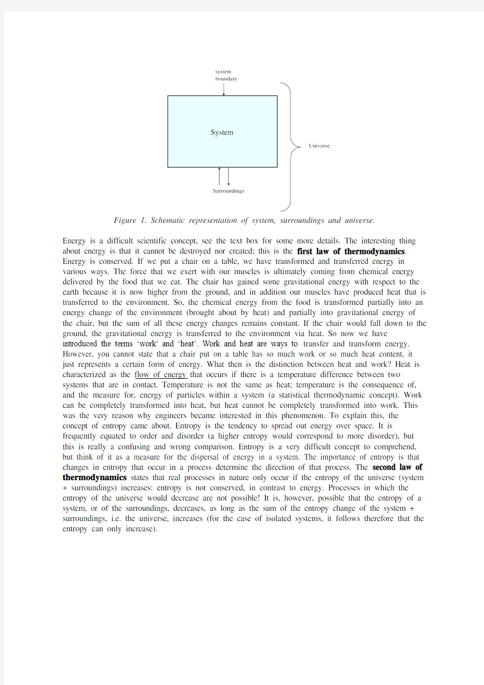
First, we need to consider some basic concepts, of systems, surroundings, energy, heat and work, and, most importantly, entropy. In thermodynamics you always need to define a system and the boundary with its surroundings: see Figure 1. The total of system + surroundings is the universe. A system can be anything: a molecule, a crystal, an emulsion droplet, a food, a factory, the earth, anything you like as long as you define it well. Systems can be subdivided in:

-Isolated systems: no exchange of matter nor energy with the surroundings possible

-Closed systems: exchange of energy is possible but not exchange of matter with surroundings -Open systems: exchange of both energy and matter with surroundings is possible

An example of an isolated system in relation to foods would be a Dewar flask with hot coffee (though in real life a Dewar flask is not completely isolated; eventually the coffee will become cold). A closed system would be a can of sterilized food, an open system a freshly baked bread put on a table: it will cool down (exchange of energy with surroundings) and it will lose water (exchange of matter with the surroundings).

1 / 15

about energy is that it cannot be destroyed nor created; this is the first law of thermodynamics. Energy is conserved. If we put a chair on a table, we have transformed and transferred energy in various ways. The force that we exert with our muscles is ultimately coming from chemical energy delivered by the food that we eat. The chair has gained some gravitational energy with respect to the earth because it is now higher from the ground, and in addition our muscles have produced heat that is transferred to the environment. So, the chemical energy from the food is transformed partially into an energy change of the environment (brought about by heat) and partially into gravitational energy of the chair, but the sum of all these energy changes remains constant. If the chair would fall down to the ground, the gravitational energy is transferred to the environment via heat. So now we have introduced the terms ‘work’ and ‘heat’. Work and heat are ways to transfer and transform energy. However, you cannot state that a chair put on a table has so much work or so much heat content, it just represents a certain form of energy. What then is the distinction between heat and work? Heat is characterized as the flow of energy that occurs if there is a temperature difference between two systems that are in contact. Temperature is not the same as heat; temperature is the consequence of, and the measure for, energy of particles within a system (a statistical thermodynamic concept). Work can be completely transformed into heat, but heat cannot be completely transformed into work. This was the very reason why engineers became interested in this phenomenon. To explain this, the concept of entropy came about. Entropy is the tendency to spread out energy over space. It is frequently equated to order and disorder (a higher entropy would correspond to more disorder), but this is really a confusing and wrong comparison. Entropy is a very difficult concept to comprehend, but think of it as a measure for the dispersal of energy in a system. The importance of entropy is that changes in entropy that occur in a process determine the direction of that process. The second law of thermodynamics states that real processes in nature only occur if the entropy of the universe (system + surroundings) increases: entropy is not conserved, in contrast to energy. Processes in which the entropy of the universe would decrease are not possible! It is, however, possible that the entropy of a system, or of the surroundings, decreases, as long as the sum of the entropy change of the system + surroundings, i.e. the universe, increases (for the case of isolated systems, it follows therefore that the entropy can only increase).

Lecture-notes-module-2

3 / 15

Lecture-notes-module-2

This finding that with every process the entropy of the universe must increase has important consequences. The second law gives the direction of processes and it also puts a limit on how much heat (the flow of energy due to a temperature difference) can be transformed to work (work however, can be completely turned into heat). What is the importance of this for predicting food quality? Well, if we know entropy changes of processes that occur in foods, we can predict the direction and the extent of these changes. But how can we estimate entropy changes? This is where Gibbs comes in. It is all about energy and entropy changes, but the changes depend on conditions of temperature T, pressure P, volume V. Energy is usually indicated with the symbol U and entropy with the symbol S. In real life, it is not always convenient to work with the concept of energy U. Other concepts have therefore been defined such as enthalpy (symbol H), which is equivalent to the energy change due to heat at constant pressure P:

(1a)

or:

(1b)

The symbol Δ refers to a change, from a certain starting point to an end point of a process. In thermodynamics we are only interested in changes, not in absolute values. But in order to calculate changes we need reference values. These are called standard states. They are defined at the condition of P = 1 bar and T C (this is only a convention and in principle arbitrary, it could be any other value). Standard states are indicated by the superscript o. So, if you see the symbol ΔH o it means that this enthalpy change refers to standard conditions.

If ΔH < 0 we speak about an exothermic reaction (energy is transferred as heat from the system to the environment), if ΔH > 0 we speak about an endothermic reaction (energy is transferred as heat from the environment to the system).

Another derived quantity is the already announced Gibbs free energy, to be considered at constant temperature and pressure:

(2a)

or:

(2b)

The importance of the Gibbs energy is as follows. As mentioned above, the second law stipulates that processes only can occur if the entropy of the universe increases. It is however not well possible to measure entropy changes of the universe, but Gibbs derived (not shown here) that the requirement that the entropy of the universe should increase is equivalent to the requirement that ΔG < 0. (Gibbs energy is sometimes also called free energy because numerically it equals the maximum useful work that a process can do exclusive of P d V work.) So, if we are able to calculate ΔG for a certain process, then we can predict whether that process can take place or not, namely only if ΔG < 0.

How can we calculate these ΔG values? Due to the many experiments done in the past, values for enthalpy, entropy and Gibbs energy changes have been determined for all kinds of components and they are listed in handbooks, such as the Handbook of Chemistry and Physics. Since equilibrium thermodynamics is only concerned about differences in begin and end state, we can calculate ΔG values without having to be concerned on how that end state is actually achieved.

5 / 15

As for the energy content of foods, see Textbox 3.

Lecture-notes-module-2

Now we are equipped to evaluate the significance of ΔG in the prediction of whether or not reactions are possible and to what extent. More specifically, we move now to chemical thermodynamics, which is about energy and entropy changes of chemical reactions. The key quantity in chemical thermodynamics is the so-called chemical potential. As the word suggests, it indicates the potential of a chemical compound to do something (to react, to move). Formally the chemical potential (symbol μ) is defined as:

(3)

This shows that the chemical potential of a component i is basically the molar Gibbs free energy, it indicates how the Gibbs free energy of a component changes if the number of moles n i of that component is changed. Without giving the derivation, a link can be made between the chemical potential and the experimentally accessible concentration of a component i in a solution:

(4)

μi o is the chemical potential at standard conditions (e.g., c i 1 mol L, C), R is the gas constant and T absolute temperature (K). However, this equation is only valid for so-called ideal solutions (no interactions between solvent and solute). To keep the simple relationship of equation (4) for non-ideal solutions, concentration c i is replaced by activity a i.

(5)

Activity is related to concentration (where the relation depends on the measurement scale): for the molarity scale (c i in mol/L) (6)

for the molality scale (m i in mol/kg solvent) (7)

for the mole fraction scale (X i is dimensionless) (8)

y i, γi and f i are the so-called molar, molal and rational activity coefficients, respectively. It is important to realize that the numerical values of activity coefficients depend on the scale used. Incidentally, every food science student should be familiar with the activity concept because of the notion of water activity a w. This is the same thermodynamic concept, in which the activity of water a w as a solvent is expressed in the mole fraction scale and the relation with the chemical potential of water is then:

(9)

Water activity can be measured experimentally from vapour pressure P w above a solution and P* above pure water:

(10)

In real life situations, certainly also for foods, we do not have ideal solutions, so the use of activity coefficients is really necessary. Only in the case that the value of activity coefficients = 1, concentrations can be used, otherwise activities should be used. Activity coefficients can differ quite strongly from unity, they can be smaller but also higher than 1. Unfortunately, activity coefficients cannot (yet) be predicted from theory (except for ion solutions) and therefore they must be determined experimentally. It is also important to realize that some analytical methods determine activities rather than concentrations, such as pH and ion-specific electrodes, osmotic measurements and water activity measurements. Methods such as titration and spectroscopy, on the other hand, determine numbers of molecules (i.e., concentrations) and do not yield information on activities.

7 / 15

Now, we can make a move to chemical reactions. Remember that our goal is to predict changes that occur in foods. Let us assume first the course of the most simple reaction where a reagent

A turns into a product P:

(11)

We are interested in the direction of this reaction as a function of the presence of A and P, and to what extent the reaction proceeds. We know already that a reaction is only possible if ΔG is negative. How do we relate this ΔG to the reaction? From equation (3) it follows that:

(12)

We now want to investigate how G changes if a change in composition takes place due to the chemical reaction, and therefore we introduce the concept of extent of reaction ξ:

(13)

In this general equation, υi reflect the stoichiometric coefficients. For our simple reaction of equation (11) it follows that

(14) Then, it follows that

(15)

and

(16)

This derivative is frequently indicated as the reaction Gibbs energy , which is a bit unfortunate because it hides the fact that it is really a differential equation, but as long as you are aware of it there is no problem. Because we can relate chemical potentials to concentrations/activities, equation (16) shows that the change in reaction Gibbs free energy is experimentally accessible. If we now consider equation (11) in conditions of the standard state of 1mol per litre, and assume that the reactant and product remain in this condition (which is hypothetical, we relax this assumption in a moment), we can picture this situation as in Figure 2. To be sure, in this picture G P o is assumed to be higher than

G A o but this can also be the other way around.

Lecture-notes-module-2

stay under standard conditions.

The slope of the line in Figure 2 is the standard reaction Gibbs energy and this is a constant (in this case positive) value. This parameter will turn out to be an important one.

However, reactants and products do not need to be in standard conditions, and also if a reactant starts to react, it cannot remain in standard condition because its concentration necessarily changes and mixing with product P will occur. As soon as mixing takes place, this results in an entropy increase (more microstates become accessible). It can be derived (not shown here) that the Gibbs free energy decrease and entropy increase due to mixing for an ideal solution is:

(17)

(18)

in which X A and X P reflect the mole fraction of A and P, respectively, and . This equation shows that the Gibbs free energy and entropy change due to mixing are minimal and maximal at a mole fraction of X A=0.5 for an ideal solution in which the enthalpy of mixing is zero: see Figure 3. However, other effects also determine the change in Gibbs free energy, namely the difference in standard entropy and enthalpy, and this is the reason that the equilibrium position will usually not be at the position where the entropy of mixing is maximal. It is the combination of enthalpy, entropy and temperature that determines the equilibrium, which is expressed in the Gibbs free energy. We therefore need to study till what point the Gibbs free energy G will decrease, in other words when becomes negative so that the reaction will proceed until : see Figure 4.

9 / 15

i

(indicating the number of molecules involved in the reaction):

(19) It can be derived that (as a generalization of equation 16):

(20) Note, again, that is a derivative, not a difference! It can next be derived for the hypothetical

reaction in equation (20) that:

Lecture-notes-module-2

11 / 15

(21)

We have introduced yet another parameter Q , the reaction quotient. Note that this reaction quotient is determined by activities, not concentrations! If these activities can be measured, we can calculate Q . Equation (22) reflects that there are concentration dependent (reflected in RT ln Q ) and concentration independent contributions (reflected in ) to the change in reaction free energy. As stated before, at equilibrium =0, and the composition of the reaction mixture at equilibrium is commonly indicated by the equilibrium constant K , in other words, at equilibrium Q = K , hence:

(22)

Equilibrium constants have been determined for many reactions and can be looked up. Please note that can be positive and negative, it should not be confused with ΔG or that can only be negative for a reaction to proceed! If < 0, it means that the equilibrium constant K > 1 (products will be favoured in the equilibrium position), and conversely if > 0, it means that K < 1

(reactants will be favoured at equilibrium). That is why in Figure 3 the equilibrium lies more in the direction of reactant than product, because > 0. For a given T , is a fixed value, whereas is determined by and the concentrations of reactants and products, as nicely summarized in equation (21). The following equation as well as Table 1 summarize what we have discussed so far. (23)

As a reminder, at the point where =0, this corresponds to the situation that the free energy is minimized under the conditions applied. So, we are finally there what we wanted to achieve: being able to predict in which direction a reaction will go and to what extent. There is a lot of confusion and mistakes in the literature about the differences between ,

, ΔG , and it is essential that you understand the differences! To be complete, a reaction for which is named an endergonic reaction, while for < 0, it is called an exergonic reaction.

As food technologists, it is interesting to know how we could influence reactions. The above analysis shows that we can play with concentrations of reactants and products to steer a reaction in a certain reaction. Another option is to change the temperature (and for reactions in the gas phase, also the pressure). The effect of temperature on an equilibrium constant is expressed in the van ‘t Hoff equation:

(24)

First of all, this equation reminds us that the equilibrium position is determined by both enthalpy and entropy changes that occur during the reaction. However, the temperature dependence of the

equilibrium constant is determined by enthalpy changes only, as the following analysis shows:

(25)

So, a plot of ln K versus 1/T should be a straight line where the slope is determined by ΔH o. Another interesting point that follows from the van ‘t Hoff equation is the following. Remember that for an exothermic reaction, ΔH o is negative, and the van ‘t Hoff equation then predicts that K will decrease with increasing temperature, in other words reactants are more favoured than products if the temperature is increased; the opposite is true for endothermic reactions: more products will be formed at higher temperatures.

In terms of the influence of enthalpy and entropy on the direction of reactions, Table 2 gives some general guidelines.

D H D S D G

Negative

(exothermic)

Positive Always negative: reaction from left to right at all temperatures

Negative (exothermic) Negative Negative at low temperature: reaction from left to right Positive at high temperature: reaction from right to left

Positive (endothermic) Positive Positive at low temperature: reaction from right to left

Negative at high temperature: reaction from left to right

Positive

(endothermic)

Negative Positive at all temperatures: reaction only from right to left

1)referring to the reaction going from left to right

It is worthwhile to elaborate a bit further on the equilibrium constant K in the light of activities. As shown in eqn 21 K (or Q for that matter)is determined by activities, not by concentrations. In practice, however, concentrations are used, and by replacing activities by concentrations and activity coefficients, it becomes clear that practical equilibrium constants K c are not really constants, while thermodynamic equilibrium constants K t are:

(26)

Activity coefficients change with concentrations, but because K t is a true constant, it implies that K c has to change with concentrations as well, and thus are not real constants!

It should be clear from this discussion that it is important to work with activities rather than with concentrations. This is particularly true for charged compounds, such as salt anions and cations, proteins, amino acids, organic acids. The very fact that these compounds carry a charge makes them behave non-ideal. Figure 5 gives an impression of how much activity coefficients may deviate from unity (note that activities are only equal to concentration for the case that the activity coefficient is 1).

Lecture-notes-module-2

In the case of charged molecules, theory is available to calculate the magnitude of activity coefficients as a function of ionic strength. For very simple and dilute systems we have the limiting law of the Debye-Hückel theory (not suited for practical systems), the extended Debije-Hückel theory, and the empirical Davies equation. A more modern version is the so-called Mean Spherical Approximation (MSA) theory, which is also taking non-ideal behaviour of non-charged molecules into account. For instance, Figure 6 shows an example how the uncharged component sucrose has an effect on the pH of a salt solution. This can be explained by the MSA theory: the presence of sucrose changes the environment for the salt ions: less volume is available for them, and this results in an increased activity of the H+ ions. So, the decrease in pH shown in Figure 4 is not due to more H+ ions, but due to the fact that they become more active!

Figure 6. Effect of sugar on the pH of a salt solution.

For the purpose of this course we only consider the Debije-Huckel and the Davies equation. These equations express the numerical value of activity coefficients. The parameters that are needed are the valencies z of the ions, the ionic strength I, and the so-called Debije-Hückel constants A and B (which are, by the way, temperature dependent). The ionic strength I is defined as;

(27)

The Debije-Hückel limiting law (only valid for I < 0.01 M):

(28)

The extended Debije-Hückel law (only valid for I < 0.1 M):

(29)

The parameter d represents the ion diameter. At 25 oC, the numerical values of A = 0.51 and B =

0.329.

The Davies equation, valid for I < 0.3, is:

(30)

The symbol stands for the mean ionic activity coefficient; this parameter is introduced because it is not possible to measure experimentally activity coefficients for individual ions. The mean ion activity coefficient for the cation with valency p and the anion with valency q is defined as:

(31) Figure 7 shows an example of how the mean ionic activity coefficient of NaCl depends on the ionic strength and how the above mentioned models fit to the experimental data.

Lecture-notes-module-2

activity models (solid line: Davies equation, dotted line: limiting DH equation, dotted-hyphenated line: extended DH equation).

Activity coefficients are of importance in the calculation of ion association, solubility calculations, dissociation of acids and bases.

Some literature references

Quilez, J. First-year university chemistry textbooks’ misrepresentation of Gibbs energy. J. Chem Ed. 89(2012)87-93

Van Boekel, MAJS. Chapter 3 and 6 in Kinetic modelling of reactions in foods. CRC/Taylor & Francis, Boca Raton, 2008.

Walstra, P. Physical Chemistry of Foods. New York, Marcel Dekker, 2003.

De Levie, R. On teaching ionic activity effects: What, when and where. J. Chem. Ed. 82 (2005) 878- 884

Th. Bindel. Understanding chemical equilibrium using entropy analysis: the relationship between

ΔS tot (sys o) and the equilibrium constant. J. Chem. Ed. 87(2010)694-699

15 / 15