Global budget of methanol Constraints from atmospheric observations

Global budget of methanol:Constraints from atmospheric observations

Daniel J.Jacob,1Brendan D.Field,1Qinbin Li,1,2Donald R.Blake,3Joost de Gouw,4

Carsten Warneke,4Armin Hansel,5Armin Wisthaler,5Hanwant B.Singh,6

and A.Guenther7

Received28June2004;revised5January2005;accepted2February2005;published26April2005.

[1]We use a global three-dimensional model simulation of atmospheric methanol to

examine the consistency between observed atmospheric concentrations and current

understanding of sources and sinks.Global sources in the model include128Tg yrà1from

plant growth,38Tg yrà1from atmospheric reactions of CH3O2with itself and other

organic peroxy radicals,23Tg yrà1from plant decay,13Tg yrà1from biomass burning

and biofuels,and4Tg yrà1from vehicles and industry.The plant growth source is a

factor of3higher for young than from mature leaves.The atmospheric lifetime of

methanol in the model is7days;gas-phase oxidation by OH accounts for63%of the

global sink,dry deposition to land26%,wet deposition6%,uptake by the ocean5%,and

aqueous-phase oxidation in clouds less than1%.The resulting simulation of atmospheric concentrations is generally unbiased in the Northern Hemisphere and reproduces the

observed correlations of methanol with acetone,HCN,and CO in Asian outflow.

Accounting for decreasing emission from leaves as they age is necessary to reproduce

the observed seasonal variation of methanol concentrations at northern midlatitudes.

The main model discrepancy is over the South Pacific,where simulated concentrations are

a factor of2too low.Atmospheric production from the CH3O2self-reaction is the

dominant model source in this region.A factor of2increase in this source(to50–100Tg

yrà1)would largely correct the discrepancy and appears consistent with independent

constraints on CH3O2concentrations.Our resulting best estimate of the global source of

methanol is240Tg yrà1.More observations of methanol concentrations and fluxes are

needed over tropical continents.Better knowledge is needed of CH3O2concentrations in

the remote troposphere and of the underlying organic chemistry.

Citation:Jacob,D.J.,B.D.Field,Q.Li,D.R.Blake,J.de Gouw,C.Warneke,A.Hansel,A.Wisthaler,H.B.Singh,and A.Guenther(2005),Global budget of methanol:Constraints from atmospheric observations,J.Geophys.Res.,110,D08303, doi:10.1029/2004JD005172.

1.Introduction

[2]Methanol is the second most abundant organic gas in the atmosphere after methane.It is present at typical con-centrations of1–10ppbv in the continental boundary layer and0.1–1ppbv in the remote troposphere[Singh et al., 1995;Heikes et al.,2002].It is a significant atmospheric source of formaldehyde[Riemer et al.,1998;Palmer et al., 2003a]and CO(B.N.Duncan et al.,Global model study of the interannual variability and trends of carbon monoxide (1988–1997):1.Model formulation,evaluation,and sensi-tivity,submitted to Journal of Geophysical Research,2004, hereinafter referred to as Duncan et al.,submitted manu-script,2004),as well as a minor term in the carbon cycle [Heikes et al.,2002]and in the global budgets of tropo-spheric ozone and OH[Tie et al.,2003].Most of the observations of atmospheric methanol concentrations con-sist of short-term records in surface air[Heikes et al.,2002]. Recent aircraft missions have added a new dimension to our knowledge of methanol concentrations in the global tropo-sphere[Singh et al.,2000,2001,2003a,2004;Lelieveld et al.,2002].We use here a global3-D chemical transport model(CTM)to examine the constraints that these aircraft observations provide on current understanding of methanol sources and sinks.

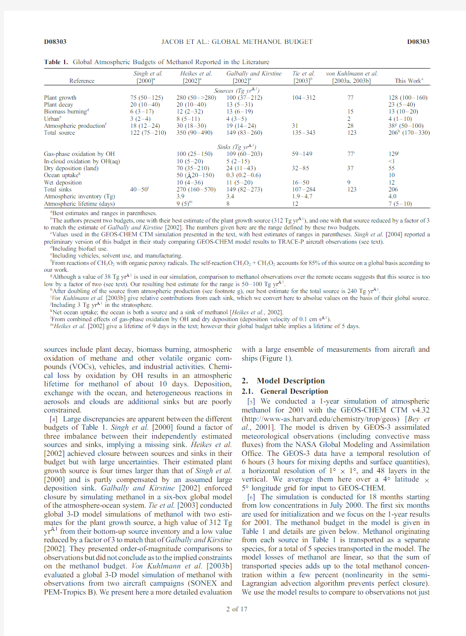
[3]Global budgets of atmospheric methanol have been presented previously by Singh et al.[2000],Galbally and Kristine[2002],Heikes et al.[2002],Tie et al.[2003],and von Kuhlmann et al.[2003a,2003b].They are summarized in Table1.Plant growth is the principal source.Additional

JOURNAL OF GEOPHYSICAL RESEARCH,VOL.110,D08303,doi:10.1029/2004JD005172,2005 1Division of Engineering and Applied Science,Harvard University,

Cambridge,Massachusetts,USA.

2Now at Jet Propulsion Laboratory,Pasadena,California,USA.

3Department of Chemistry,University of California,Irvine,California,

USA.

4NOAA Aeronomy Laboratory,Boulder,Colorado,USA.

5Institute of Ion Physics,University of Innsbruck,Innsbruck,Austria.

6NASA Ames Research Center,Moffett Field,California,USA.

7Atmospheric Chemistry Division,National Center for Atmospheric

Research,Boulder,Colorado,USA.

Copyright2005by the American Geophysical Union.

0148-0227/05/2004JD005172$09.00

sources include plant decay,biomass burning,atmospheric oxidation of methane and other volatile organic com-pounds(VOCs),vehicles,and industrial activities.Chemi-cal loss by oxidation by OH results in an atmospheric lifetime for methanol of about10days.Deposition, exchange with the ocean,and heterogeneous reactions in aerosols and clouds are additional sinks but are poorly constrained.

[4]Large discrepancies are apparent between the different budgets of Table1.Singh et al.[2000]found a factor of three imbalance between their independently estimated sources and sinks,implying a missing sink.Heikes et al. [2002]achieved closure between sources and sinks in their budget but with large uncertainties.Their estimated plant growth source is four times larger than that of Singh et al. [2000]and is partly compensated by an assumed large deposition sink.Galbally and Kirstine[2002]enforced closure by simulating methanol in a six-box global model of the atmosphere-ocean system.Tie et al.[2003]conducted global3-D model simulations of methanol with two esti-mates for the plant growth source,a high value of312Tg yrà1from their bottom-up source inventory and a low value reduced by a factor of3to match that of Galbally and Kirstine [2002].They presented order-of-magnitude comparisons to observations but did not conclude as to the implied constraints on the methanol budget.Von Kuhlmann et al.[2003b] evaluated a global3-D model simulation of methanol with observations from two aircraft campaigns(SONEX and PEM-Tropics B).We present here a more detailed evaluation with a large ensemble of measurements from aircraft and ships(Figure1).

2.Model Description

2.1.General Description

[5]We conducted a1-year simulation of atmospheric methanol for2001with the GEOS-CHEM CTM v4.32 (https://www.wendangku.net/doc/5912081097.html,/chemistry/trop/geos)[Bey et al.,2001].The model is driven by GEOS-3assimilated meteorological observations(including convective mass fluxes)from the NASA Global Modeling and Assimilation Office.The GEOS-3data have a temporal resolution of 6hours(3hours for mixing depths and surface quantities), a horizontal resolution of1°?1°,and48layers in the vertical.We average them here over a4°latitude?5°longitude grid for input to GEOS-CHEM.

[6]The simulation is conducted for18months starting from low concentrations in July2000.The first six months are used for initialization and we focus on the1-year results for2001.The methanol budget in the model is given in Table1and details are given below.Methanol originating from each source in Table1is transported as a separate species,for a total of5species transported in the model.The model losses of methanol are linear,so that the sum of transported species adds up to the total methanol concen-tration within a few percent(nonlinearity in the semi-Lagrangian advection algorithm prevents perfect closure). We use the model results to compare to observations not just

Table1.Global Atmospheric Budgets of Methanol Reported in the Literature

Reference Singh et al.

[2000]a

Heikes et al.

[2002]a

Galbally and Kirstine

[2002]a

Tie et al.

[2003]b

von Kuhlmann et al.

[2003a,2003b]This Work c

Sources(Tg yrà1)

Plant growth75(50–125)280(50–>280)100(37–212)104–31277128(100–160) Plant decay20(10–40)20(10–40)13(5–31)23(5–40) Biomass burning d6(3–17)12(2–32)13(6–19)1513(10–20) Urban e3(2–4)8(5–11)4(3–5)24(1–10) Atmospheric production f18(12–24)30(18–30)19(14–24)312838g(50–100) Total source122(75–210)350(90–490)149(83–260)135–343123206h(170–330)

Sinks(Tg yrà1)

Gas-phase oxidation by OH100(25–150)109(60–203)59–14977i129j

In-cloud oxidation by OH(aq)10(5–20)5(2–15)<1

Dry deposition(land)70(35–210)24(11–43)32–853755

Ocean uptake k50(à20–150)0.3(0.2–0.6)10

Wet deposition10(4–36)11(5–20)16–50912

Total sinks40–50l270(160–570)149(82–273)107–284123206 Atmospheric inventory(Tg) 3.9 3.4 1.9–4.7 4.0 Atmospheric lifetime(days)9(5)m8127(5–10)

a Best estimates and ranges in parentheses.

b The authors present two budgets,one with their best estimate of the plant growth source(312Tg yrà1),and one with that source reduced by a factor of3 to match the estimate of Galbally and Kirstine[2002].The numbers given here are the range defined by these two budgets.

c Values use

d in th

e GEOS-CHEM CTM simulation presented in the text,with best estimates o

f ranges in parentheses.Singh et al.[2004]reported a preliminary version of this budget in their study comparin

g GEOS-CHEM model results to TRACE-P aircraft observations(see text).

d Including biofuel use.

e Including vehicles,solvent use,and manufacturing.

f From reactions of CH

3O2with organic peroxy radicals.The self-reaction CH3O2+CH3O2accounts for85%of this source on a global basis according to

our work.

g Although a value of38Tg yrà1is used in our simulation,comparison to methanol observations over the remote oceans suggests that this source is too low by a factor of two(see text).Our resulting best estimate for the range is50–100Tg yrà1.

h After doubling of the source from atmospheric production(see footnote g),our best estimate for the total source is240Tg yrà1.

i Von Kuhlmann et al.[2003b]give relative contributions from each sink,which we convert here to absolue values on the basis of their global source. j Including3Tg yrà1in the stratosphere.

k Net ocean uptake;the ocean is both a source and a sink of methanol[Heikes et al.,2002].

l From combined effects of gas-phase oxidation by OH and dry deposition(deposition velocity of0.1cm sà1).

m Heikes et al.[2002]give a lifetime of9days in the text;however their global budget table implies a lifetime of5days.

from 2001but from other years as well,assuming that interannual variability is a relatively small source of error.[7]Correlations of the methanol simulation with consis-tent simulations of CO,HCN,and acetone for 2001are also presented for comparison with ship and aircraft observa-tions.The CO and HCN simulations are as described by Li et al.[2003].The acetone simulation is as described by Jacob et al.[2002]but without an ocean source (for reasons to be discussed in section 4.2).

2.2.Sources of Methanol 2.2.1.Plant Growth

[8]We use the plant physiology model of Galbally and Kirstine [2002]in which methanol emission scales as net primary productivity (NPP)with emission factors per unit carbon of 0.020%for grasses and 0.011%for other plants.This offers a process-based parameterization for global mapping of the methanol source from plant growth.We apply the emission factors to a monthly NPP database from the CASA 2biosphere model with 1°?1°spatial resolution [Potter et al.,1993;Randerson et al.,1997].The global NPP in that database is 17Pg C yr à1for grasslands and 41Pg C yr à1for other plants.The resulting methanol emission is 128Tg yr àhttps://www.wendangku.net/doc/5912081097.html,parison to previous studies in Table 1would suggest at least a factor of 2uncertainty on this global source but our simulation of atmospheric obser-vations implies a narrower range,as discussed later.

[9]The Galbally and Kirstine [2002]relationship of methanol emission to NPP has yet to be tested with field observations,and NPP estimates are themselves subject to substantial uncertainty [Karl et al.,2004].Our initial

simulations used monthly mean NPP values to distribute methanol emissions seasonally,but there resulted large model overestimates of observed methanol concentrations at northern midlatitudes in late summer and https://www.wendangku.net/doc/5912081097.html,boratory and field data indicate in fact that methanol emissions from young leaves are a factor of 2–3higher than from mature leaves [McDonald and Fall ,1993;Nemecek-Marshall et al.,1995;Karl et al.,2003].We fit these results by scaling our monthly mean NPP-based emissions with the following parameterization adapted from A.Guenther:

a i ?

b 1t2max L i àL i à1

L i

;0

e1T

where L i is the local leaf area index for month i ,a i is the monthly scaling factor,and b is a normalizing factor such

that

P

12i ?1

a i =12for each grid square.The normalization ensures consistency with the Galbally and Kirstine [2002]

NPP-based algorithm on a yearly basis.Leaf area indices in the model are computed monthly as a function of ecosystem type,NPP,and global vegetation index (GVI),following the algorithm of Guenther et al.[1995]as implemented by Wang et al.[1998].The resulting methanol emissions at midlatitudes peak in spring,when they may be as much as a factor of three larger than in summer.Within a given month we distribute the methanol source evenly over the daytime hours,assuming zero emission from green plants at night [Nemecek-Marshall et al.,1995;Schade and Goldstein ,2001;Warneke et al.,

2002].

Figure 1.Atmospheric observations of methanol used for comparison with model results.Ship cruises indicated by lines include INDOEX over the Indian Ocean in March 1999[Wisthaler et al.,2002]and AOE-2001over the Arctic Ocean in July August 2001(A.Hansel and A.Wisthaler,unpublished data,2001).Aircraft missions indicated by lines include TRACE-P over the North Pacific in March–April 2001[Singh et al.,2003a,2004]and TOPSE over the North American Arctic in February–May 2000(D.R.Blake,unpublished data,2000).Additional aircraft missions indicated by boxes include SONEX over the North Atlantic in October–November 1997(regions 1–2)[Singh et al.,2000],MINOS over the eastern Mediterranean in August 2001(region 3)[Lelieveld et al.,2002],ITCT 2K2over the northeast Pacific in April–May 2002(region 4)[Nowak et al.,2004],and PEM-Tropics B over the South Pacific in February–March 1999(regions 5–9)[Singh et al.,2001].The symbol labeled ‘‘10’’indicates the locations of Innsbruck (Austria)[Holzinger et al.,2001]and Zugspitze (Germany,2650m ASL)(A.Hansel and A.Wisthaler,unpublished data,2003),both at (47N,11E).

2.2.2.Plant Decay

[10]Warneke et al.[1999]reported the abiotic emission of methanol from decaying plant matter with an emission factor of3–5?10à4g per g of C oxidized.We apply this emission factor to monthly mean heterotrophic respiration rates with1°?1°resolution from the CASA2model.The global heterotrophic respiration rate is58Pg C yrà1and the resulting methanol source is17–29Tg yrà1(best estimate 23Tg yrà1).Galbally and Kirstine[2002]point out that part of the methanol produced by plant decay may be consumed within the litter,but they also point out that additional biotic processes contribute to the methanol source from plant decay.Their best estimate for the total source from plant decay is13Tg yrà1(range5–31).

2.2.

3.Biomass Burning and Biofuels

[11]We use a methanol/CO emission factor of0.018mol molà1for combustion of different types of biomass,based on compilations of literature data[Yokelson et al.,1999; Andreae and Merlet,2001].Yokelson et al.[1999]find little variability in the emission factor between different types of fires(range0.006–0.031mol molà1).Singh et al.[2004] find a mean emission factor of0.016±0.002mol molà1for fire plumes from Southeast Asia sampled over the NW Pacific.Christian et al.[2003]find a mean value of 0.024mol molà1for Indonesian fuels.Holzinger et al. [2004]find a mean value of0.038mol molà1for aged biomass burning plumes sampled over the Mediterranean Sea,which is relatively high and which they attribute to secondary production;but the fire plumes sampled by Singh et al.[2004]were also aged.

[12]We apply the0.018mol molà1emission factor to gridded CO emission inventories for biomass burning (climatological,monthly)[Duncan et al.,2003]and bio-fuels(aseasonal)[Yevich and Logan,2003].Global emis-sions in these inventories are440Tg CO yrà1for biomass burning and161Tg CO yrà1for biofuels,and the resulting methanol sources are9and4Tg yrà1respectively.Inverse modeling estimates of the global biomass burning source of CO constrained with surface air observations fall in the range600–740Tg CO yrà1[Bergamaschi et al.,2000; Pe′tron et al.,2002],about50%higher than used here. 2.2.4.Urban

[13]We refer to‘‘urban’’as the ensemble of methanol sources from fossil fuel combustion,other vehicular emissions,solvents,and industrial activity[Galbally and Kirstine,2002].We use the aseasonal gridded(1°?1°) EDGAR V2.0global anthropogenic emission inventory for1990,which gives a total urban alkanol emission of 8.2Tg yrà1[Olivier et al.,1994],and assume that methanol accounts for half of this total or4.1Tg yrà1.Goldan et al. [1995]reported a concentration ratio of methanol to nitro-gen oxides(NO x)of0.17mol molà1in urban air in Colorado in winter;scaling of this source to a global fossil fuel combustion NO x source of23Tg N yrà1would yield an anthropogenic source of methanol of9.1Tg yrà1. Aircraft measurements by J.deGouw(unpublished)indi-cate methanol/CO enhancement ratios of0.050mol molà1 in Denver but0.011–0.014mol molà1in other U.S.cities. An emission ratio of0.013mol molà1,combined with a global fossil fuel source of CO of480Tg yrà1(Duncan et al., submitted manuscript,2004),would imply a global methanol source of7.1Tg yrà1.Holzinger et al.[2001]report a methanol:benzene enhancement ratio of0.8mol molà1for urban air in Innsbruck,Austria.The EDGAR V2.0inventory gives a global benzene emission of1.2Tg yrà1from vehicles and industry,which would imply a methanol source of only 0.4Tg yrà1.The urban source of methanol is thus highly uncertain but is clearly small on a global scale.

2.2.5.Atmospheric Production

[14]Methanol is produced in the atmosphere by reactions of the methylperoxy(CH3O2)radical with itself and with higher organic peroxy(RO2)radicals[Madronich and Calvert,1990;Tyndall et al.,2001]:

CH3O2tCH3O2!CH3OHtCH2OtO2

eR1T

CH3O2tRO2!CH3OHtR0CHOtO2

eR2T

Alternate branches for these reactions,not producing methanol,are

CH3O2tCH3O2!CH3OtCH3OtO2

eR10T

CH3O2tRO2!CH3OtROtO2

eR20T

The CH3O2and RO2radicals are produced in the atmosphere by oxidation of VOCs.The sum of reactions (R1),(R10),(R2),and(R20)typically accounts for less than 10%of the CH3O2sink in current chemical mechanisms. The dominant atmospheric sinks are the reactions with HO2 and NO,which do not produce methanol:

CH3O2tHO2!CH3OOHtO2

eR3T

CH3O2tNO!CH3OtNO2

eR4T

[15]We calculate the atmospheric source of methanol from(R1)and(R2)with a GEOS-CHEM simulation of tropospheric ozone-NO x-VOC chemistry[Fiore et al., 2003].Primary VOCs in that simulation include methane, ethane,propane,higher alkanes,>C2alkenes,isoprene, acetone,and methanol.The simulation uses recommended data from Tyndall et al.[2001]for the kinetics and methanol yields of(R1),and also for(R3)involving the acetonylperoxy radical(CH3C(O)CH3O2)produced by oxidation of acetone. The methanol yields at298K for these two reactions are0.63 and0.5,respectively.We assume a0.5yield for all other CH3O2+RO2reactions,following Madronich and Calvert [1990].The resulting global source of methanol is38Tg yrà1. Reaction(R1)contributes85%of that global total.The remaining15%,contributed by(R2),mainly involves RO2 radicals produced from biogenic isoprene and is largely confined to the continental boundary layer,where it is much smaller than the primary emission from plant growth.In the remote atmosphere,where the atmospheric production of methanol is of most interest,the CH3O2 radicals driving(R1)originate mainly from the oxidation of methane.

[16]Previous literature estimates of the atmospheric source of methanol from(R1)and(R2),similarly obtained with global tropospheric chemistry models,are in the range

18–31Tg yrà1(Table1),lower than our estimate.These include30Tg yrà1from Heikes et al.[2002]computed with an earlier version of GEOS-CHEM.Discrepancies between estimates reflect differences in the abundances of NO and HO2,the CH3O2reaction rate constants,the yield of methanol from(R1)and(R2),and the importance of (R2).Uncertainties in the(R1)rate constant and in the corresponding methanol yield are each about30%at298K [Tyndall et al.,2001]and higher at colder temperatures.As we will see,observations from the PEM-Tropics B aircraft mission over the South Pacific suggest an even larger atmospheric source of methanol than is used here.

2.3.Sinks of Methanol

2.3.1.Gas-Phase Oxidation by OH

[17]We use the rate constant k=3.6?10à12exp[à415/T] cm3moleculeà1sà1recommended by Jimenez et al.[2003] with an uncertainty of20%.We apply this rate constant to a 3-D archive of monthly mean OH concentrations from the Fiore et al.[2003]GEOS-CHEM simulation of tropospheric ozone-NO x-VOC chemistry.The lifetime of methylchloro-form against tropospheric oxidation by OH(proxy for the global mean tropospheric OH concentration)is5.6years in that simulation[Martin et al.,2003].This is within the range constrained by the methylchloroform observations,which imply a25%uncertainty in global mean OH concentrations [Intergovernmental Panel on Climate Change(IPCC), 2001].Stratospheric loss of methanol is computed using OH concentrations archived from a global2-D stratospheric chemistry model[Schneider et al.,2000]and amounts to only2%of the loss in the troposphere.Our computed lifetime of methanol against oxidation by OH is11days. Addition of errors in quadrature implies an uncertainty of 30%on this value.

2.3.2.Aqueous-Phase Oxidation by OH(aq)

[18]Methanol dissolves in aqueous aerosols(Henry’s law constant H=1.6?10à5exp[4900/T]M atmà1)and can then be oxidized by OH(aq)(k=1.0?109exp[à590/T] Mà1sà1;Elliot and McCracken[1989]).The corresponding first-order loss rate constant(sà1)for atmospheric methanol is k0=HLRTk[OH(aq)]where L is the dimensionless liquid water content,R is the gas constant,and[OH(aq)]is the OH(aq)concentration in units of M(moles per liter of water).The reaction takes place mainly in clouds,where L is more than3orders of magnitude higher than in a clear-sky atmosphere.The GEOS-3meteorological archive pro-vides3-D cloud optical depths t from which we estimate L= 4t r/3Q D Z where r is the effective cloud droplet radius(taken to be10m m),Q%2is the cloud droplet extinction efficiency, and D Z is the vertical thickness of the gridbox.The OH(aq) concentration in cloud droplets is largely determined by aqueous-phase cycling with HO2(aq)/O2àand depends in a complicated way on cloud composition[Jacob,1986].We assume here a simple parameterization[OH(aq)]=d[OH(g)] where[OH(g)]is the gas-phase concentration calculated in GEOS-CHEM without consideration of aqueous-phase cloud chemistry,and d=1?10à19M cm3moleculeà1is chosen to fit the cloud chemistry model results of Jacob[1986].The resulting lifetime of methanol against in-cloud oxidation by OH(aq)is longer than1year.Heikes et al.[2002]and Galbally and Kirstine[2002]found a larger role for in-cloud oxidation by OH(aq)in their global methanol budgets,amounting to5–10%of the gas-phase loss (Table1).Their assumed OH(aq)concentrations and aqueous-phase CH3OH+OH rate constants are higher than ours.

[19]A few studies have raised the possibility of a missing heterogeneous sink for methanol in aerosols or clouds.Singh et al.[2000]suggested that such a sink might explain their observed decrease of methanol con-centrations from the middle to upper troposphere at north-ern midlatitudes(SONEX aircraft mission).Jaegle′et al. [2000]found that unexpectedly high formaldehyde con-centrations measured in the upper troposphere during SONEX correlated with methanol,and speculated that reactive uptake of methanol in cirrus clouds with a reaction probability g=0.01could provide an explanation.Yokelson et al.[2003]observed the depletion of methanol in a cloud polluted by biomass burning smoke,and Tabazadeh et al. [2004]proposed that surface reactions of methanol on cloud droplets could be responsible.However,statistical compari-son of in-cloud versus clear-sky methanol concentrations in the large data set from the TRACE-P aircraft mission indi-cates no significant differences at any altitude[Singh et al., 2004].Upper tropospheric observations from the SONEX mission indicate no depletion in air processed by deep convection or cirrus clouds[Jaegle′et al.,2000].Laboratory studies indicate no significant reactive uptake of methanol by sulfuric acid aerosols[Iraci et al.,2002],ice[Hudson et al.,2002;Winkler et al.,2002],or mineral oxide surfaces [Carlos-Cuellar et al.,2003].Kane and Leu[2001]report fast reaction of methanol with sulfuric acid in concen-trated solutions but Iraci et al.[2002]attribute this result to an experimental artifact.At present,the weight of evidence does not support a fast heterogeneous sink for methanol.

2.3.3.Deposition to Land

[20]Microbial and foliar uptake of methanol by vegeta-tion and soils is difficult to separate from the plant growth and decay sources,either observationally or for model purposes.Investigators have placed soil and leaf litter [Schade and Goldstein,2001]and foliage[Nemecek-Marshall et al.,1995]in enclosures and observed a net emission of methanol.However,these studies used enclo-sures that were flushed with methanol-free air.Recent measurements by A.Guenther(unpublished)indicate that there can be a net uptake of methanol when enclosures are flushed with air containing ambient levels of methanol. [21]Measurement of the diurnal cycle of methanol con-centrations at continental surface sites provides some sepa-ration of microbial uptake from plant growth emission, which is restricted to daytime.Kesselmeier et al.[2002] observed no significant diurnal variation at a site in the Amazon forest,but other observations at sites in the tropics and northern midlatitudes indicate decreases over the course of the night ranging from about30%[Goldan et al.,1995]to several-fold[Riemer et al.,1998;Holzinger et al.,2001; Karl et al.,2004],suggesting surface uptake.A30% decrease over the course of an8-hour summer night,and for a typical nighttime mixing depth of100m,would imply a methanol deposition velocity of0.12cm sà1.Karl et al. [2004]measured methanol deposition to a tropical forest ecosystem by using a combination of eddy covariance and vertical gradients,and found a mean methanol deposition

velocity of0.27±0.14cm sà1.On the basis of the above information,and acknowledging the large uncertainty,we assume here a constant dry deposition velocity of0.2cm sà1 to land.We assume that this deposition velocity also applies to ice-covered surfaces since Boudries et al.[2002]found that Arctic snow is a net sink for methanol.The resulting atmospheric lifetime of methanol against dry deposition is 26days.Including a methanol sink from dry deposition improves significantly the ability of the model to reproduce observations at northern midlatitudes in fall and winter. 2.3.4.Wet Deposition

[22]We simulate wet deposition of methanol with the GEOS-CHEM wet deposition scheme described by Liu et al.[2001].This scheme accounts for scavenging of water-soluble species by convective updrafts,convective anvils, and large-scale precipitation.The scavenging coefficients used by Liu et al.[2001]are scaled here to the dissolved fraction of methanol inferred from the local liquid water content and Henry’s law constant.Scavenging is assumed to take place in warm clouds only(T>268K).The retention efficiency of methanol upon cloud droplet freezing is taken to be0.02,by analogy with previous assumptions for CH3OOH and CH2O[Mari et al.,2000],so that scavenging is ineffi-cient in mixed liquid-ice clouds where the precipitation involves https://www.wendangku.net/doc/5912081097.html,boratory studies indicate that methanol coverage of ice surfaces is low,less than10à4of a monolayer at equilibrium[Hudson et al.,2002;Winkler et al.,2002], supporting the assumption of a low retention efficiency.The resulting lifetime of methanol against wet deposition is 120days.With such a long lifetime,wet deposition does not significantly affect the vertical profile of methanol in the troposphere[Crutzen and Lawrence,2000].

2.3.5.Uptake by the Ocean

[23]Simple solubility considerations imply that the ocean mixed layer must be a large reservoir for methanol[Galbally and Kirstine,2002;Singh et al.,2003a].Heikes et al.[2002] point out that methanol is both produced and consumed in the ocean.Singh et al.[2003a]observed a gradient of increasing methanol concentrations from the marine boundary layer to the free troposphere over the remote North Pacific during TRACE-P,implying an ocean sink with a mean deposition velocity of0.08cm sà1.Measurements taken at the Mace Head coastal site in Ireland also show evidence of methanol uptake by the ocean,with a similar deposition velocity [Carpenter et al.,2004].Our GEOS-CHEM results presented in the work of Singh et al.[2003a]show that an ocean saturation ratio of90%for methanol,combined with a standard two-layer parameterization of ocean-atmosphere exchange,gives a good simulation of the observed TRACE-P vertical gradients.In the absence of better infor-mation we assume that the90%saturation ratio holds globally.The resulting lifetime of methanol against net uptake by the ocean is130days.

3.Global Model Budget and Atmospheric Distribution of Methanol

[24]Table1summarizes our global model budget of methanol.The global source of206Tg yrà1includes contributions from plant growth(62%),atmospheric oxida-tion of VOCs(18%),plant decay(11%),biomass burning and biofuels(6%),and vehicles and industrial activities (2%).The global sink balancing that source is dominated by gas-phase oxidation by OH(63%)with minor contributions from dry deposition to land(26%),wet deposition(6%),net uptake by the ocean(5%),and aqueous-phase oxidation in clouds(<1%).The resulting atmospheric lifetime of meth-anol is7days and the global atmospheric burden is4.0Tg.

A preliminary version of our model budget was presented by Singh et al.[2004]in a study comparing GEOS-CHEM results to their TRACE-P aircraft observations(reference to our budget is given there as B.D.Field et al.,manuscript in preparation,2003).That preliminary version did not include deposition of methanol to land or the dependence of methanol emissions on leaf age.

[25]Our global source of methanol is in the range of previous literature cited in Table1(122–350Tg yrà1). Differences reflect principally the magnitude of the plant growth source.Our value for that source(128Tg yrà1)is close to that of Galbally and Kirstine[2002](100Tg yrà1), as would be expected since we followed their algorithm. Our atmospheric source of methanol from CH3O2reactions (38Tg yrà1)is larger than previous estimates(18–31Tg yrà1).

[26]Gas-phase oxidation by OH is a major methanol sink in all the inventories of Table1.However,the principal methanol sink in the Heikes et al.[2002]budget is dry deposition to land and oceans,with an assumed deposition velocity of0.4cm sà1.As mentioned above,the TRACE-P aircraft data of Singh et al.[2003a]imply a much lower deposition velocity to the ocean.Fast deposition to land in the Heikes et al.[2002]budget(90Tg yrà1)partly com-pensates for their high terrestrial biogenic source(280Tg yrà1).The relative contributions to the methanol sink from gas-phase oxidation by OH,dry deposition,and wet depo-sition in our model are essentially the same as in the previous global3-D model study by von Kuhlmann et al. [2003a](63%,30%,and7%respectively).That study did not report separate deposition terms to land and ocean. [27]Figure2shows the mean concentrations of methanol simulated by the model in surface air and at500hPa,for January and July.Surface air concentrations over land exceed5–10ppbv in the tropics and at northern midlatitudes in summer.The particularly high concentrations over Siberia in July are due to the long continental fetch and the late emergence of leaves.Surface air concentrations at northern midlatitudes in winter drop to0.5–2ppbv.Concentrations over land decrease typically by a factor of2–5from the surface to500hPa,reflecting the surface source and the7-day lifetime.There is by contrast little vertical gradient over the oceans.Concentrations over the northern hemi-sphere oceans(0.5–1ppbv)show little seasonal variation, because faster chemical loss in summer balances the effect of the larger continental source.Concentrations over the south-ern hemisphere oceans are higher in winter(0.5–1ppbv) than in summer(0.2–0.5ppbv)since the continental source in the southern hemisphere is mainly in the tropics and has little seasonal variation.Concentrations are lowest(below 0.2ppbv)in surface air over Antarctica in summer.

4.Evaluation With Observations

[28]We examine in this section how the above estimates of methanol sources and sinks,when implemented in a

global CTM,succeed in reproducing the observed atmo-spheric concentrations of methanol.Our primary focus is on observations from aircraft and ships,which integrate source information over large regions.Observations from surface continental sites,reviewed by Heikes et al.[2002],are few and show high spatial variability that we cannot expect to reproduce given our crude model representation of sources.We use these surface observations mainly to examine large-scale features,including seasonal variations and tropical concentrations,that are of particular interest for testing the model.

4.1.Surface Concentrations

[29]The review of Heikes et al.[2002]gives representa-tive surface air concentrations of 20(range 0.03–47)ppbv in urban air,10(1–37)ppbv over forests,6(4–9)ppbv over grasslands,2(1–4)ppbv for continental background,and 0.9(0.3–1.4)ppbv over the northern hemispheric oceans.Our model values are roughly consistent with these ranges,as shown in Figure 2.Urban air is not resolved on the scale of the model.

[30]The Heikes et al.[2002]compilation includes no surface data for tropical land ecosystems,where the model predicts high concentrations year-round.Measurements by Kesselmeier et al.[2002]in the Rondo ?nia tropical forest of Brazil (10S,63W)for a 7-day period in October 1999(end of dry season)indicate a range of 1to 6ppbv.Our mean

simulated concentration for that site and month is much higher,10ppbv,with dominant contributions from plant growth (6ppbv),plant decay (2ppbv),and biomass burning (2ppbv).Measurements by Karl et al.[2004]at a tropical forest site in Costa Rica (10N,84W)for a 20-day period in April–May 2003(peak of dry season)indicate a mean concentration of 2.2ppbv.Our mean simulated concentra-tion for that site and 2-month period is 2.1pppbv,in agreement with observations,with a major contribution from plant growth (1.2ppbv)and minor contributions of about 0.3ppbv each from plant decay,biomass burning,and atmospheric production.The lower model value in Costa Rica than in Rondo ?nia reflects the shorter continental fetch.The model shows little seasonal variation at the Rondo ?nia site (monthly means range from 8to 10ppbv)but more at the Costa Rica site (1.2to 2.7ppbv).At the latter site,the seasonal maximum is in the wet season (June–October)when the plant growth source is high,and the seasonal minimum is in the early dry season (January–February)before biomass burning.Karl et al.[2004]also made methanol flux measurements at the Costa Rica site,which indicate a value 50%higher than the parameterization of Galbally and Kristine [2002]when normalized to the estimated tropical forest NPP.On the other hand,the data from Kesselmeier et al.[2002]would suggest that the NPP-based parameterization of Galbally and Kristine [2002]is too high for the Amazon forest.More observations

of

Figure 2.Simulated monthly mean concentrations of methanol (ppbv)in surface air and at 500hPa for January and July 2001.

methanol concentrations and fluxes are clearly needed for tropical land ecosystems.

[31]To our knowledge,the only methanol observations in the literature extending over a full yearly cycle are those of Holzinger et al.[2001]taken in the outskirts of Innsbruck,Austria (47N,11E).These authors used concurrent mea-surements of benzene (emitted by vehicles)to separate the local urban from the regional nonurban components of methanol.Figure 3shows the observed ranges for the nonurban component.There is a spring-summer maximum and fall-winter minimum,reflecting biogenic emission.Concentrations drop by more than a factor of 2from June to September.Also shown in Figure 3are the simulated methanol concentrations and the contributions from the individual model sources.Plant growth is the main model source except in winter,when plant decay and urban sources become relatively important.The model reproduces the seasonal variation in the observations,including the rise from winter to spring and the decrease from spring to fall.The latter reflects in the model the weaker emission from mature leaves.

[32]Ship measurements from Wisthaler et al.[2002]over the Indian Ocean during INDOEX 1999(March 1999)provide another important data set for methanol in surface air.The cruise track extended from 20N to 12S,starting from the west coast of India and extending south of the intertropical convergence zone (Figure 1).Observed meth-anol concentrations exceed 1ppbv in Indian outflow and drop to 0.5–0.6ppbv in southern hemispheric air.Wisthaler et al.[2002]reported a strong correlation of methanol with CO,which we compare in Figure 4to our mean monthly model results for 2001sampled along the cruise track.The agreement is remarkably good.The model captures

the

Figure 3.Seasonal variation of methanol concentrations at Innsbruck,Austria.The ranges of observations reported by Holzinger et al.[2001]for different times of year in 1996–1997are shown as vertical lines with symbols.These observations are for the non-urban component of methanol,after subtraction of the urban component based on correlation with benzene.Model results are shown as the solid line,with additional lines identifying contributions from individual sources in the model:plant growth (short dashes),plant decay (dots),urban (thin solid),biomass burning and biofuels (long dashes),and atmospheric production

(dash-dot).

Figure 4.Methanol-CO correlations along the INDOEX 1999cruise track over the Indian Ocean (Figure 1).Observations from Wisthaler et al.[2002]are shown as small dots,with linear regression as solid line.Monthly mean GEOS-CHEM results along the cruise track are shown as large open circles,with linear regression as dashed line.Coefficients of determination (r 2)and slopes of the linear regressions (S )are shown inset.

clean 0.5–0.6ppbv background and the observed relation-ship with CO,although it does not capture the population of observations with relatively high CO but low methanol (hence the stronger methanol-CO correlation in the model,r 2=0.76versus r 2=0.47).Over India in the model the methanol is mostly from plant growth,while CO is mostly from combustion;the methanol-CO correlation in Indian outflow reflects varying degrees of dilution with the marine background rather than a commonality of methanol and CO source processes.

[33]Additional unpublished methanol measurements have been made by A.Wisthaler and A.Hansel on a ship cruise in the Arctic in July August 2001(AOE-2001),and at Zugspitze in southern Germany (47N,11E,2650m altitude)for four months in October 2002to January 2003.These are shown in Figure 5together with the corresponding model results.The model reproduces the low Arctic cruise obser-vations north of 85N (0.30–0.35ppbv),reflecting deposi-tion to the ocean,but not the even lower concentrations (0.1–0.2ppbv)observed further south;these low concen-trations are from only a few measurements and suggest a strong local ocean sink.Observations at Zugspitze show a decrease from 0.7ppbv in October to 0.3ppbv in January.The model also shows a decrease,mostly from the deposi-tion sink,but not as strong as observed.This would suggest a nonphotochemical sink of methanol missing from the model.However,the TOPSE aircraft observations over the North American Arctic in winter,to be discussed in section 4.3,show higher concentrations than at Zugspitze and do not suggest such a missing sink.

https://www.wendangku.net/doc/5912081097.html,n Outflow (TRACE-P Mission)

[34]The TRACE-P aircraft mission in March–April 2001provided extensive data for methanol and other species in

Asian outflow over the North Pacific [Jacob et al.,2003].The outflow included a major contribution from seasonal biomass burning in Southeast Asia [Heald et al.,2003a].Flight tracks are shown in Figure 1.Our model simulation is for the same meteorological year as TRACE-P.We sample the model along the flight tracks and for the flight days for comparison to observations.GEOS-CHEM simu-lations for the TRACE-P period have been evaluated previously with observations for a number of species including in particular CO [Kiley et al.,2003;Palmer et al.,2003b]and HCN [Li et al.,2003],which we discuss below in the context of their correlations with methanol.The model gives a good simulation of Asian outflow pathways with no evident transport bias [Liu et al.,2003;I.Bey et al.,Characterization of transport errors in chemical forecasts from a global tropospheric chemical transport model,submitted to Journal of Geophysical Research ,2005].Simulation of the CO 2observations indicates a 45%underestimate of the net biospheric carbon emission for China in the CASA 2model during the TRACE-P period [Suntharalingam et al.,2004].However,as we will see below,there is no evident bias in our methanol simulation.

4.2.1.Vertical Profiles

[35]Figure 6compares the mean simulated and observed vertical profiles of methanol concentrations for the four TRACE-P quadrants separated at 30N,150E.The four quadrants contrast fresh Asian outflow west of 150E to more background North Pacific air to the east.

[36]The observed methanol concentrations in the NW quadrant decrease from 1.5–2ppbv in the boundary layer to 0.9–1.3ppbv in the free troposphere,rise again to a maximum in excess of 2ppbv in the upper troposphere,and then decline to 0.1ppbv above the tropopause at 12

km.

Figure 5.Mean methanol concentrations from the AOE-2001Arctic cruise in July August 2001as a function of latitude and from Zugspitze (southern Germany,2650m ASL)in October 2002to January 2003as a function of month.Unpublished observations from A.Wisthaler and A.Hansel (closed circles)are compared to model results (open circles).Standard deviations on the observations are shown for Zugspitze.

The model reproduces these features although it is up to a factor 2too low in the middle troposphere.Stratospheric concentrations cannot be compared because of excessive stratosphere-troposphere exchange in the GEOS assimilat-ed meteorological data used to drive the model [Liu et al.,2001;Tan et al.,2004].The plant growth source in the model contributes a relatively featureless background of 0.3ppbv throughout the troposphere in this NW quadrant.The boundary layer enhancement reflects a mix of Chi-nese emissions from plant decay,biofuels,and urban sources.The upper tropospheric enhancement is due to outflow from deep convection in Southeast Asia and is contributed mainly by the plant growth and biomass burning components.

[37]The observed mean profile for the SW quadrant in Figure 6shows greater influence from Southeast Asia than the NW quadrant.Concentrations decrease gradually with altitude,from 1.5ppbv in the boundary layer to 0.5–1ppbv in the middle and upper troposphere but with a convective enhancement apparent at 8–9km.The model reproduces this structure with no evident bias.

[38]Observations in the NE quadrant show a marked increase with altitude,in contrast to the western https://www.wendangku.net/doc/5912081097.html,n influence is principally in the middle and upper troposphere.The model underestimates this Asian influ-ence,by about the same factor as for the free tropospheric Asian outflow in the NW quadrant.The relatively low methanol concentrations in the lower troposphere,both in the model and in the observations,reflect gas-phase oxida-tion and ocean uptake of methanol as the Asian air masses subside [Singh et al.,2003a].

[39]Asian influence during TRACE-P was weakest in the SE quadrant,which lies south of the dominant outflow track.The observed layer of high methanol concentrations at 2–4km altitude is from one single Hawaii-Guam flight where the aircraft sampled repeatedly an Asian outflow plume that had traveled southward and subsided [Crawford et al.,2004].High CO concentrations (200ppbv)were observed in that layer.Previous analysis of the GEOS-CHEM CO simulation shows that this layer is displaced upward and diluted in the model relative to the observations [Heald et al.,2003b].A similar bias is found for methanol,as the model enhancement is at 4–5km altitude and peaks at only 0.7ppbv.The model is also low in the marine boundary layer (0.4ppbv,versus 0.6ppbv in the observa-tions);atmospheric production is the most important model source there and is probably too weak,as discussed later in the context of the PEM-Tropics B observations over the South Pacific.

[40]Singh et al.[2004]previously compared results from our preliminary model version (not including dry deposition to land or the decrease in the plant growth source as leaves age)to their mean observed background vertical profile of methanol concentrations for the ensemble of the mission.This showed agreement within 10%up to 6km altitude,but a growing model overestimate at higher altitudes (up to a factor of 3at 11km)that they speculated could reflect heterogeneous chemical loss not captured by the model.

In

Figure 6.Vertical profiles of methanol concentrations from the TRACE-P aircraft mission over the North Pacific (March–April 2001)averaged over four quadrants separated at 30N,150E (Figure 1).Means and standard deviations of observations are shown as symbols and horizontal lines;the number of observations contributing to each average is indicated.Model results are shown as solid lines,with additional lines identifying contributions from individual model sources:plant growth (short dashes),plant decay (dots),urban (thin solid),biomass burning and biofuels (long dashes),and atmospheric production (dash-dot).

the Singh et al.[2004]comparison,observed methanol concentrations decrease from 0.8ppbv at 6km to 0.35ppbv at 11km (filtered against stratospheric influence);whereas model values increase from 0.9ppbv at 6km to 1.1ppbv at 11km.Our comparisons in Figure 6do not show such a model bias in the upper troposphere,but instead consider-able regional difference in simulated and observed vertical profiles for the different quadrants,as discussed above.The decreasing trend from 6to 11km in the observations is found only for the southern quadrants.In addition,the model values presented here are lower than in the prelim-inary simulation reported by Singh et al.[2004]due to our subsequent inclusion of a land deposition sink in the model.This affects in particular the simulation of upper tropospheric concentrations,which include a major contribution from convective outflow of tropical continental air.4.2.2.Correlations With Other Species

[41]Further insight can be gained by examining the observed correlations of methanol with other species.In the ensemble of TRACE-P observations we find that methanol correlates most strongly with acetone (r 2=0.83,slope =0.38mol mol à1),HCN (r 2=0.78,slope =0.12mol mol à1),and CO (r 2=0.63,slope =64mol mol à1).These correlations are shown in Figure 7.The slopes are given

with methanol as denominator.We generated corresponding correlations from the model results sampled along the flight tracks.These are also shown in Figure 7.The CO and HCN simulations are as described in the work of Li et al.[2003].The acetone simulation presented here is that of Jacob et al.[2002]applied to the TRACE-P period,but without an ocean source since the TRACE-P observations indicate that the ocean was in fact a net sink for acetone [Singh et al.,2003a].We find that an ocean source for acetone in the model would destroy the correlation with methanol since the ocean is a sink for methanol.

[42]The model reproduces the correlation between meth-anol and acetone found in the observations (r 2=0.49,slope =0.48mol mol à1in the model).The biogenic acetone source in the model is scaled to isoprene emission [Jacob et al.,2002],while that of methanol is scaled to NPP.The stronger correlation in the observations suggests that the sources of acetone and methanol are governed by more similar processes than is assumed in the model.Measure-ments at rural U.S.sites in summer have previously shown a strong correlation between acetone and methanol with an acetone/methanol slope of 0.21–0.27mol mol à1[Goldan et al.,1995;Riemer et al.,1998].The higher slope observed here is due to anthropogenic sources of

acetone.

Figure 7.Correlations of methanol with CO,acetone,and HCN concentrations in the ensemble of TRACE-P data.Observations (top panels)are compared to model results (bottom panels).Coefficients of determination (r 2),regression lines,and corresponding slopes (S )are indicated.

[43]The observed correlation between methanol and HCN is well simulated by the model(r2=0.43,slope= 0.10mol molà1).The dominant source of HCN variability in the TRACE-P data is biomass burning in Southeast Asia [Li et al.,2003;Singh et al.,2003b].The observed HCN/ CO molar emission ratio from biomass burning varies in the literature over a large range from0.03%to1.1%,with a best fit for the TRACE-P conditions of0.27%[Li et al.,2003]. Combined with our estimated methanol/CO molar emission ratio from biomass burning of1.8%mol molà1this yields an HCN/methanol emission ratio of0.15mol molà1.The weaker slope in the model and in the observations likely reflects biogenic methanol emissions in Southeast Asia that are collocated with the biomass burning emissions. [44]Good agreement between model and observations is also found in the correlation of methanol with CO(r2= 0.44,slope=69mol molà1in the model).CO here serves as a general tracer of Asian outflow and the correlation mainly provides support for the overall magnitude of methanol export from the Asian continent.Although the model underestimates the TRACE-P methanol observations in the middle troposphere(Figure6),the methanol-CO correlation is principally driven by strong outflow events in the boundary layer[Liu et al.,2003].

4.3.Other Aircraft Observations

[45]We now compare model results to methanol obser-vations from other aircraft missions including TOPSE at North American high latitudes in February–May2000 (D.R.Blake,unpublished data),SONEX over the North Atlantic in October–November1997[Singh et al.,2000], MINOS over the eastern Mediterranean in August2001 [Lelieveld et al.,2002],ITCT2K2over the Northeast Pacific in April–May2002[Nowak et al.,2004],and PEM-Tropics B over the South Pacific in February–March 1999[Singh et al.,2001].Aside from MINOS,these missions were conducted for years other than the2001 model year.We use monthly mean vertical profiles in the model over the flight regions(Figure1)to compare to the mean observations.The measurements in TRACE-P, SONEX,and PEM-Tropics B were made by real-time gas chromatography(GC).The measurements in ITCT2K2and MINOS were made by proton transfer mass spectrometry (PTR-MS).A ship-based intercomparison of online PTR-MS and real-time GC-MS methods indicates high correla-tion between the two and agreement within a few percent [de Gouw et al.,2003].Calibration differences of up to20% may be expected between the GC measurements of Singh et al.from different missions.The TOPSE measurements were made by GC analysis from collected air canisters,all with the same relative humidity and the same lapse of time between collection and analysis.The accuracy is estimated to be30%and the precision is much better.

[46]Additional aircraft methanol data are available from the PEM-West B mission over the NW Pacific in February–March1994[Singh et al.,1995]and from the LBA-CLAIRE mission over the rain forest in Surinam in March 1998[Williams et al.,2001].The PEM-West B data are from the same region and season as TRACE-P,and show similar concentrations[Singh et al.,2004],but represent a much sparser data set.The LBA-CLAIRE data indicate low methanol concentrations,averaging1.1ppbv in the bound-ary layer and0.6ppbv in the free troposphere.These would suggest,consistent with Kesselmeier et al.[2002],that methanol emission from tropical forests of South America is much lower than predicted from the Galbally and Kirstine [2002]parameterization.However,quantitative comparison to the model is difficult because the observations were

taken https://www.wendangku.net/doc/5912081097.html,titudinal profiles of methanol concentrations at North American high latitudes during the TOPSE mission(Figure1),for February and April and for0–2and4–6km altitude.Mean observations

(D.R.Blake,unpublished data,2000)are shown as solid circles;the number of observations used to compute the mean is also shown.Model results are shown as open circles.

under conditions of marine inflow and only about 12hours downwind of the coast.

[47]The TOPSE measurements are of particular interest as they characterize the latitudinal gradient at high northern latitudes during the transition from winter to spring [Atlas et al.,2003].We show in Figure 8the latitudinal profiles measured at 0–2and 4–6km altitude in February and April (only a few observations are available in May).Also shown are the corresponding model profiles,sampled as monthly means along the TOPSE flight tracks.Boundary layer concentrations in February show a latitudinal decrease from 1ppbv at northern midlatitudes to 0.4ppbv in the Arctic,both in the model and the observations,due to the shutting down of the biogenic source and the effect of surface deposition.The same latitudinal gradient is found in April but concentrations are about 0.2ppbv higher,similarly in the model and in the observations,reflecting the springtime source.Concentrations at 4–6km altitude show by contrast little latitudinal gradient,which the model explains as reflecting a weaker influence of the dry deposition sink.The February observations at 4–6km (0.5ppbv)are higher than the wintertime Zugspitze observations discussed in section 4.1and are more consistent with the model results.

The model misses the observed April enhancement at 4–6km south of 60N although it captures it in the 0–2km data;this could be due to model error in the springtime onset of the source.We have no explanation for the high concentrations (above 1ppbv)observed north of 80N at 4–6km in April.

[48]Aircraft observations at northern midlatitudes are available from the SONEX,MINOS,and ITCT 2K2mis-sions.These are shown in Figure 9together with the corresponding model results.Observed concentrations in the middle and upper troposphere in SONEX are low,0.4ppbv on average,and this is reproduced in the model with only a slight positive bias.Reduced methanol emission from mature leaves is critical for simulation of the SONEX observations;without this reduction the simulated methanol concentrations would be much higher in fall because of the weak photochemical sink.The global 3-D model study of von Kuhlmann et al.[2003b]also found good agreement with the SONEX observations using a global methanol source 40%lower than ours (Table 1).They did not account for the decrease of methanol emission with leaf age.

[49]The model reproduces the free tropospheric concen-trations observed in MINOS (0.6–1ppbv)over the

Medi-

Figure 9.Vertical profiles of methanol concentrations from the SONEX,MINOS,ITCT 2K2,and PEM-Tropics B aircraft missions averaged over the regions of Figure 2.Symbols and lines are as for Figure 6.The MINOS observations are taken from Lelieveld et al.[2002]without information on the number of observations.

terranean in July,and also the high values in surface air.It is too low in the lower free troposphere(2–4km),possibly reflecting difficulties in simulating vertical mixing and transport over this highly heterogeneous region.Salisbury et al.[2003]observed a mean concentration of3.3ppbv at a site in Crete during MINOS,and as shown in Figure9this is consistent with model https://www.wendangku.net/doc/5912081097.html,parisons to the von Kuhlmann et al.[2003a,2003b]model presented in that paper found it to be too low by a factor of four on average, possibly reflecting its low plant growth source.

[50]Observations from the ITCT2K2campaign off the California coast in April–May average0.9–1.1ppbv in the 1–7km column with lower values near the surface, consistent with an ocean sink.The model is0.2–0.6ppbv too low.The comparison near the surface is subject to uncertainty because of land-ocean contrast(the model has more continental influence than the observations,but this may be due to numerical diffusion).The free tropospheric observations in ITCT2K2are similar in magnitude to the TRACE-P observations for the northeast quadrant (Figure6),but the model shows lower values in ITCT 2K2because of the longer distance from the Asian conti-nent.Atmospheric production makes a relatively large contribution(0.2ppbv)to the simulated concentrations in ITCT2K2,reflecting the strong radiation and low NO x concentrations over the subsiding northeast Pacific.A possibility,discussed further below,is that this atmospheric source in the model is too weak.

[51]Observations from the PEM-Tropics B campaign over the South Pacific are typically0.6–1.2ppbv with little horizontal or vertical structure(Figure9).These values are remarkably high considering the remoteness from land.The model is about a factor of2too low, averaging about0.4–0.5ppbv with little structure.A unique feature of model results for this region is that atmospheric production is the dominant source,contribut-ing0.2–0.4ppbv.This source is favored by the high UV radiation(stimulating CH3O2production),low NO x con-centrations(suppressing competition from the CH3O2+NO reaction),and low CO/CH4ratio(resulting in a high CH3O2/HO2ratio).The model underestimate in this region suggests that atmospheric production in the model is too low.A doubling of this source would largely correct the discrepancy and would be consistent with the featureless character of the observations.

[52]We previously discussed in section2the uncertain-ties in computing the atmospheric source of methanol from CH3O2reactions.Examination of model results for the PEM-Tropics(B)region indicates that self-reaction(R1) accounts for5–10%of the CH3O2sink,reaction(R4)with NO for20%,and reaction(R3)with HO2for the rest; reaction(R2)is negligible.CH3OOH produced by(R3)has an atmospheric lifetime of about a day against losses by reaction with OH and photolysis:

CH3OOHtOH!CH3O2tH2O

eR5aT

CH3OOHtOH!CH2OtOHtH2O

eR5bT

CH3OOHth n!CH3OtOH

eR6T

[53]Reaction(R5a)recycles CH3O2while reactions (R5b)and(R6)do not.For typical atmospheric conditions, (R5a)accounts for about50%of CH3OOH loss and(R5b) and(R6)each for about25%.Assuming chemical steady state for CH3OOH,the effective sink of CH3O2from(R3)is determined by k3(1àf),where the CH3O2recycling efficiency f=k5a/(k5a+k5b+k6)is about50%.Jet Propulsion Laboratory(JPL)[2003]gives uncertainty esti-mates of30%for k3,40%for k5,and50%for k6(it gives no uncertainty estimate for the recommended branching ratio 70/30for k5a/k5b).Thus the overall uncertainty on the effective CH3O2sink from(R3)could be a factor of two. In addition,Martin et al.[2002]showed that the NO concentrations simulated by GEOS-CHEM over the South Pacific are about50%higher than the PEM-Tropics(B) https://www.wendangku.net/doc/5912081097.html,bination of these two factors could easily allow a doubling of the source of methanol from(R1), considering that this source is quadratic in the CH3O2 concentration.Photochemical model calculations by Olson et al.[2001]along the PEM-Tropics(B)flight tracks indicated a50%overestimate of observed CH3OOH,which would be consistent with an overestimate of(R3).They also indicated a factor of2underestimate of CH2O(common product of CH3O2degradation pathways)[Heikes et al., 2001].As discussed by Heikes et al.[2001],the latter discrepancy suggests a major contribution from VOCs other than methane to the supply of CH3O2.This would provide an alternate explanation for increasing the methanol source from the CH3O2self-reaction.

5.Discussion:Constraints on the Methanol Budget From Atmospheric Observations

[54]Observed atmospheric concentrations of methanol are consistent with the view that plant growth provides the principal global https://www.wendangku.net/doc/5912081097.html,boratory and field studies indicate a factor of2–3decrease in this source from young to mature leaves[McDonald and Fall,1993;Nemecek-Marshall et al.,1995;Karl et al.,2003].We find that this is consistent with the observed seasonal variation of meth-anol concentrations at northern midlatitudes.A global plant growth source of128Tg yrà1,computed in our model using the NPP-based algorithm of Galbally and Kirstine[2002], provides an overall unbiased simulation at northern midlat-itudes.The tropics are the largest global contributor to this source but observations there are few.Data for tropical South America[Williams et al.,2001;Kesselmeier et al., 2002]suggest that our model source is too high,while data for Costa Rica[Karl et al.,2004]are consistent with the model.More work is clearly needed to improve understand-ing of methanol emission from tropical land ecosystems. The model also predicts high surface air concentrations (>10ppbv)over Siberia in July,reflecting a large seasonal plant growth source as well as a long continental fetch. Measurements in this region would be of great value. [55]The net flux of methanol from the terrestrial bio-sphere in the model is96Tg yrà1including128Tg yrà1 from plant growth and23Tg yrà1from plant decay, balanced by55Tg yrà1dry deposition to land(Table1). The atmospheric observations offer limited constraints for separating these three different terms.The plant growth source appears to be responsible for the observed decline of

concentrations from spring to fall,while the deposition sink appears to be responsible for the observed diurnal variation of concentrations as well as the decline at northern latitudes over the course of the winter.

[56]Observed concentrations of methanol over the South Pacific during the PEM-Tropics B aircraft mission(0.6–1.2ppbv)are much higher than would be expected from the terrestrial vegetation source and show little vertical or longitudinal structure.Diffuse atmospheric production of methanol from the CH3O2self-reaction(R1),where CH3O2 originates mainly from methane oxidation,is the principal model source in the region and contributes a0.2–0.4ppbv model background.Our computed global magnitude of this source(38Tg yrà1)is larger than previous estimates(18–31Tg yrà1)but still would need to be doubled to approach the South Pacific observations.Methanol observations over the remote north tropical and subtropical Pacific(TRACE-P and ITCT2K2aircraft missions)also suggest that atmo-spheric production of methanol from(R1)in the model is too low.

[57]Computation of the methanol source from(R1)in global tropospheric chemistry models is affected by uncer-tainties in the concentration of CH3O2and in the branching ratio of CH3O2reactions.A doubling to50–100Tg yrà1 does not appear to be inconsistent with independent con-straints,and is specifically within the constraints offered by ancillary PEM-Tropics B observations of CH3OOH and CH2O.It could reflect errors in kinetic rate constants,or the presence of VOCs other than methane in the remote marine atmosphere to provide sources of CH3O2.Some observations of aldehydes in remote marine air[Heikes et al.,2001;Singh et al.,2001,2004]suggest the latter,and imply a more active organic photochemistry than is cur-rently described in models,while other observations are more consistent with current understanding[Fried et al., 2003].Measurements of HO2and total peroxy(HO2+ CH3O2+RO2)radical concentrations by the chemical amplifier method during TRACE-P indicated concentration ratios of organic peroxy radicals to HO2that are consistent with current models[Cantrell et al.,2003],but there is substantial uncertainty in these measurements.Direct mea-surements of CH3O2concentrations in the remote atmo-sphere are needed.

[58]Our model yields a global mean atmospheric lifetime for methanol of7days,with losses from gas-phase reaction with OH(63%of total loss),dry deposition to land(26%), wet deposition(6%),and uptake by the ocean(5%). Aqueous-phase oxidation by OH(aq)in clouds is negligible. The general ability of the model to reproduce the observed variability of methanol concentrations(cf.Figure7)sug-gests a relatively narrow range of uncertainty in the lifetime, 5–10days.Chemical loss of methanol by reaction with OH is uncertain by only about30%[Jimenez et al.,2003]and most likely represents the dominant global sink for metha-nol.The low methanol concentrations observed at high northern latitudes in winter imply an additional nonphoto-chemical sink,which we attribute in the model to dry deposition to land.This attribution is supported by obser-vations of methanol fluxes and of the diurnal variation of methanol concentrations at vegetated sites,although there is considerable variability from site to site.Heterogeneous loss in aerosols and clouds could provide an alternate explana-tion for the observed wintertime depletion of methanol but is not supported by independent evidence.Aircraft obser-vations of vertical profiles over the oceans suggest that ocean uptake is only a weak sink,although ship data from the AOE-2001summertime Arctic campaign suggest the possibility of rapid local uptake.Wet deposition,con-strained by the Henry’s law solubility for methanol,is only

a weak sink.

[59]Our best estimate of the global source of methanol (after allowing for doubling of atmospheric production to 76Tg yrà1)is240Tg yrà1.Singh et al.[2004]estimated a much lower global source,110Tg yrà1,by scaling the global acetone source of95Tg yrà1from Jacob et al. [2002]to the mean acetone/methanol concentration ratio of 2.1g gà1that they measured in TRACE-P and to the ratio of lifetimes of acetone(15days,from Jacob et al.[2002]) and methanol(9days,from Heikes et al.[2002]).However, the concentration ratio measured in TRACE-P is lower than the expected global mean because of the large regional anthropogenic contribution to acetone[Jacob et al.,2002] and the relatively weak biogenic methanol emission from East Asia at that time of year.A methanol source of110Tg yrà1in our model would result in a low bias relative to observations.Singh et al.[2004]acknowledge that their emission estimate is subject to large uncertainty.

6.Implications for Atmospheric Chemistry [60]Our budget implies a minor but nonnegligible role for methanol in global tropospheric chemistry.Oxidation of methanol by OH produces CH2OH(major pathway)and CH3O(minor),which both go on to produce CH2O and HO2[Jimenez et al.,2003].The global tropospheric rate of methanol oxidation calculated in our model on a per-carbon basis,47Tg C yrà1,amounts to12%of the corresponding value of380Tg C yrà1for methane oxidation[IPCC, 2001].Methanol provides a significant source of CH2O both in the continental boundary layer[Riemer et al.,1998; Palmer et al.,2003a]and in the remote troposphere[Heikes et al.,2001].The production of CO from methanol oxida-tion amounts to4–6%of the global CO source of1800–2700Tg yrà1(Duncan et al.,submitted manuscript,2004). Inclusion of methanol in GEOS-CHEM at the levels simu-lated here decreases the global tropospheric OH concentra-tion by2%,an effect similar to that reported previously by Tie et al.[2003].Regional variations in this effect on OH are discussed by Tie et al.[2003]and are relatively small.

[61]Acknowledgments.This work was funded at Harvard by the Atmospheric Chemistry Program of the U.S.National Science Founda-tion.H.B.Singh acknowledges support from the NASA IDS program.

A.Wisthaler and A.Hansel thank Caroline Leck(MISU),the coordi-nator of the Atmospheric Program of AOE-2001,and Ulrich Poeschl (TU-Munich),the coordinator of the Zugspitze SCA VEX Program.The GEOS-CHEM model is managed at Harvard University with support from the NASA Atmospheric Chemistry Modeling and Analysis Pro-gram.We thank the reviewers for their very useful comments. References

Andreae,M.O.,and P.Merlet(2001),Emission of trace gases and aerosols from biomass burning,Global Biogeochem.Cycles,15,955–966. Atlas,E.L.,B.A.Ridley,and C.A.Cantrell(2003),The Tropospheric Ozone Production about the Spring Equinox(TOPSE)Experiment: Introduction,J.Geophys.Res.,108(D4),8353,doi:10.1029/ 2002JD003172.

Bergamaschi,P.,R.Hein,M.Heimann,and P.J.Crutzen(2000),Inverse modeling of the global CO cycle:1.Inversion of CO mixing ratios, J.Geophys.Res.,105,1909–1927.

Bey,I.,D.J.Jacob,R.M.Yantosca,J.A.Logan,B.D.Field,A.M.Fiore, Q.Li,H.Liu,L.J.Mickley,and M.G.Schultz(2001),Global modeling of tropospheric chemistry with assimilated meteorology:Model descrip-tion and evaluation,J.Geophys.Res.,106,23,073–23,096. Boudries,H.,J.W.Bottenheim,C.Guimbaud,A.M.Grannas,P.B. Shepson,S.Houdier,S.Perrier,and F.Domine′(2002),Distribution and trends of oxygenated hydrocarbons in the high Arctic derived from measurements in the atmospheric boundary layer and interstitial snow air during the ALERT2000field campaign,Atmos.Environ.,36, 2573–2583.

Cantrell,C.A.,G.D.Edwards,S.Stephens,L.Mauldin,E.Kosciuch, M.Zondlo,and F.Eisele(2003),Peroxy radical observations using chemical ionization mass spectrometry during TOPSE,J.Geophys. Res.,108(D6),8371,doi:10.1029/2002JD002715.

Carlos-Cuellar,S.,P.Li,A.P.Christensen,B.J.Krueger,C.Burrichter,and V.H.Grassian(2003),Heterogeneous uptake kinetics of volatile organic compounds on oxide surfaces using a Knudsen cell reactor:Adsorption of acetic acid,formaldehyde,and methanol on a-Fe2O3,a-Al2O3,and SiO2,J.Phys.Chem.A,107,4250–4261.

Carpenter,L.J.,A.C.Lewis,J.R.Hopkins,K.A.Read,I.D.Longley,and M.W.Gallagher(2004),Uptake of methanol to the North Atlantic Ocean surface,Global Biogeochem.Cycles,18,GB4027,doi:10.1029/ 2004GB002294.

Christian,T.J.,B.Kleiss,R.J.Yokelson,R.Holzinger,P.J.Crutzen,W.M. Hao,B.H.Saharjo,and D.E.Ward(2003),Comprehensive laboratory measurements of biomass-burning emissions:1.Emissions from Indone-sian,African,and other fuels,J.Geophys.Res.,108(D23),4719, doi:10.1029/2003JD003704.

Crawford,J.H.,et al.(2004),Relationship between Measurements of Pol-lution in the Troposphere(MOPITT)and in situ observations of CO based on a large-scale feature sampled during TRACE-P,J.Geophys. Res.,109,D15S04,doi:10.1029/2003JD004308.

Crutzen,P.J.,and https://www.wendangku.net/doc/5912081097.html,wrence(2000),The impact of precipitation scavenging on the transport of trace gases:A3-dimensional model sen-sitivity study,J.Atmos.Chem.,37,81–112.

de Gouw,J.A.,P.D.Goldan,C.Warneke,W.C.Kuster,J.M.Roberts, M.Marchewka,S.B.Bertman,A.A.P.Pszenny,and W.C.Keene(2003), Validation of proton transfer reaction-mass spectrometry(PTR-MS)mea-surements of gas-phase organic compounds in the atmosphere during the New England Air Quality Study(NEAQS)in2002,J.Geophys.Res., 108(D21),4682,doi:10.1029/2003JD003863.

Duncan,B.N.,R.V.Martin,A.C.Staudt,R.Yevich,and J.A.Logan (2003),Interannual and seasonal variability of biomass burning emissions constrained by satellite observations,J.Geophys.Res.,108(D2),4100, doi:10.1029/2002JD002378.

Elliot,A.J.,and D.R.McCracken(1989),Effect of temperature on Oàreactions and equilibria:A pulse radiolysis study,Int.J.Appl.Radiat. Instrum.C,33,69–74.

Fiore,A.,D.J.Jacob,H.Liu,R.M.Yantosca,T.D.Fairlie,and Q.Li (2003),Variability in surface ozone background over the United States: Implications for air quality policy,J.Geophys.Res.,108(D24),4787, doi:10.1029/2003JD003855.

Fried,A.,et al.(2003),Airborne tunable diode laser measurements of formaldehyde during TRACE-P:Distributions and box model compari-sons,J.Geophys.Res.,108(D20),8798,doi:10.1029/2003JD003451. Galbally,I.E.,and W.Kirstine(2002),The production of methanol by flowering plants and the global cycle of methanol,J.Atmos.Chem., 43,195–229.

Goldan,P.D.,W.C.Kuster,F.C.Fehsenfeld,and S.A.Montzka(1995), Hydrocarbon measurements in the southeastern United States:The Rural Oxidants in the Southern Environment(ROSE)program1990,J.Geo-phys.Res.,100,35,945–35,963.

Guenther,A.,et al.(1995),A global model of natural volatile organic compound emissions,J.Geophys.Res.,100,8873–8892.

Heald,C.L.,D.J.Jacob,P.I.Palmer,M.J.Evans,G.W.Sachse,H.B. Singh,and D.R.Blake(2003a),Biomass burning emission inventory with daily resolution:Application to aircraft observations of Asian out-flow,J.Geophys.Res.,108(D21),8811,doi:10.1029/2002JD003082. Heald,C.L.,et al.(2003b),Asian outflow and trans-Pacific transport of carbon monoxide and ozone pollution:An integrated satellite,aircraft, and model perspective,J.Geophys.Res.,108(D24),4804,doi:10.1029/ 2003JD003507.

Heikes,B.,et al.(2001),Formaldehyde over the central Pacific during PEM-Tropics B,J.Geophys.Res.,106,32,717–32,732.

Heikes,B.G.,et al.(2002),Atmospheric methanol budget and ocean implication,Global Biogeochem.Cycles,16(4),1133,doi:10.1029/ 2002GB001895.Holzinger,R.,A.Jordan,A.Hansel,and W.Lindinger(2001),Methanol measurements in the lower troposphere near Innsbruck(047°160N; 011°240E),Austria,Atmos.Environ.,35,2525–2532.

Holzinger,R.,J.Williams,G.Salisbury,T.Klupfel,M.de Reus,M.Traub, P.J.Crutzen,and J.Lelieveld(2004),Oxygenated compounds in aged biomass burning plumes over the eastern Mediterranean:Evidence for strong secondary production of methanol and acetone,Atm.Chem.Phys. Discuss.,4,6321–6340.

Hudson,P.K.,M.A.Zondlo,and M.A.Tolbert(2002),The interaction of methanol,acetone,and acetaldehyde with ice and nitric acid-doped ice: Implications for cirrus clouds,J.Phys.Chem.,106,2882–2888. Intergovernmental Panel on Climate Change(IPCC)(2001),Climate Change2001:The Scientific Basis,edited by J.T.Houghton et al.,Cam-bridge Univ.Press,New York.

Iraci,L.T.,A.M.Essin,and D.M.Golden(2002),Solubility of methanol in low-temperature aqueous sulfuric acid and implications for atmo-spheric particle composition,J.Phys.Chem.,106,4054–4060. Jacob,D.J.(1986),The chemistry of OH in remote clouds and its role in the production of formic acid and peroxymonosulfate,J.Geophys.Res., 91,9807–9826.

Jacob,D.J.,B.D.Field,E.M.Jin,I.Bey,Q.Li,J.A.Logan,R.M. Yantosca,and H.B.Singh(2002),Atmospheric budget of acetone, J.Geophys.Res.,107(D10),4100,doi:10.1029/2001JD000694. Jacob,D.J.,J.H.Crawford,M.M.Kleb,V.S.Connors,R.J.Bendura,J.L. Raper,G.W.Sachse,J.C.Gille,L.Emmons,and C.L.Heald(2003), Transport and Chemical Evolution over the Pacific(TRACE-P)aircraft mission:Design,execution,and first results,J.Geophys.Res.,108(D20), 9000,doi:10.1029/2002JD003276.

Jaegle′,L.,et al.(2000),Photochemistry of HO x in the upper troposphere at northern midlatitudes,J.Geophys.Res.,105,3877–3892.

Jet Propulsion Laboratory(JPL)(2003),Chemical Kinetics and Photoche-mical Data for Use in Atmospheric Studies,JPL Publ.No.02–25,Jet https://www.wendangku.net/doc/5912081097.html,b.,Pasadena,Calif.

Jimenez,E.,M.K.Gilles,and A.R.Ravishankara(2003),Kinetics of the reactions of the hydroxyl radical with CH3OH and C2H5OH between235 and360K,J.Photochem.Photobiol.A,157,237–245.

Kane,S.M.,and M.-T.Leu(2001),Uptake of methanol vapor in sulfuric acid solutions,J.Phys.Chem.,105,1411–1415.

Karl,T.,A.Guenther,C.Spirig,A.Hansel,and R.Fall(2003),Seasonal variation of biogenic VOC emissions above a mixed hardwood forest in northern Michigan,Geophys.Res.Lett.,30(23),2186,doi:10.1029/ 2003GL018432.

Karl,T.,M.Potosnak,A.Guenther,D.Clark,J.Walker,J.D.Herrick,and C.Geron(2004),Exchange processes of volatile organic compounds above a tropical rain forest:Implications for modeling tropospheric chemistry above dense vegetation,J.Geophys.Res.,109,D18306, doi:10.1029/2004JD004738.

Kesselmeier,J.,et al.(2002),Concentrations and species composition of atmospheric volatile organic compounds(VOCs)as observed during the wet and dry season in Rondo?nia(Amazonia),J.Geophys.Res., 107(D20),8053,doi:10.1029/2000JD000267.

Kiley,C.M.,et al.(2003),An intercomparison and evaluation of aircraft-derived and simulated CO from seven chemical transport models during the TRACE-P experiment,J.Geophys.Res.,108(D21),8819, doi:10.1029/2002JD003089.

Lelieveld,J.,et al.(2002),Global air pollution crossroads over the Medi-terranean,Science,298,794–798.

Li,Q.,D.J.Jacob,R.M.Yantosca,C.L.Heald,H.B.Singh,M.Koike, Y.Zhao,G.W.Sachse,and D.G.Streets(2003),A global three-dimensional model analysis of the atmospheric budgets of HCN and CH3CN:Constraints from aircraft and ground measurements,J.Geophys. Res.,108(D21),8827,doi:10.1029/2002JD003075.

Liu,H.,D.J.Jacob,I.Bey,and R.M.Yantosca(2001),Constraints from 210Pb and7Be on wet deposition and transport in a global three-dimensional chemical tracer model driven by assimilated meteorological fields,J.Geophys.Res.,106,12,109–12,128.

Liu,H.,D.J.Jacob,I.Bey,R.M.Yantosca,B.N.Duncan,and G.W. Sachse(2003),Transport pathways for Asian pollution outflow over the Pacific:Interannual and seasonal variations,J.Geophys.Res.,108(D20), 8786,doi:10.1029/2002JD003102.

Madronich,S.,and J.G.Calvert(1990),Permutation reactions of organic peroxy radicals in the troposphere,J.Geophys.Res.,95,5697–5716. Mari,C.,D.J.Jacob,and P.Bechtold(2000),Transport and scavenging of soluble gases in a deep convective cloud,J.Geophys.Res.,105,22,255–22,267.

Martin,R.V.,et al.(2002),An improved retrieval of tropospheric nitrogen dioxide from GOME,J.Geophys.Res.,107(D20),4437,doi:10.1029/ 2001JD001027.

Martin,R.V.,D.J.Jacob,R.M.Yantosca,M.Chin,and P.Ginoux(2003), Global and regional decreases in tropospheric oxidants from photochemi-

cal effects of aerosols,J.Geophys.Res.,108(D3),4097,doi:10.1029/ 2002JD002622.

McDonald,R.C.,and R.Fall(1993),Detection of substantial emissions of methanol from plants to the atmosphere,Atmos.Environ.,27,1709–1713.

Nemecek-Marshall,M.,R.C.MacDonald,J.J.Franzen,C.L. Wojciechowski,and R.Fall(1995),Methanol emission from leaves,Plant Physiol.,108,1359–1368.

Nowak,J.B.,et al.(2004),Gas-phase chemical characteristics of Asian emission plumes observed during ITCT2K2over the eastern North Pacific Ocean,J.Geophys.Res.,109,D23S19,doi:10.1029/ 2003JD004488.

Olivier,J.G.J.,A.F.Bouwman,C.W.M.Van der Maas,and J.J.M. Berdowski(1994),Emission Database for Global Atmospheric Research (EDGAR),Environ.Monit.Assess.,31,93–106.

Olson,J.R.,et al.(2001),Seasonal differences in the photochemistry of the South Pacific:A comparison of observations and model results from PEM Tropics A and B,J.Geophys.Res.,106,32,749–32,766. Palmer,P.I.,D.J.Jacob,A.M.Fiore,R.V.Martin,K.Chance,and T.P. Kurosu(2003a),Mapping isoprene emissions over North America using formaldehyde column observations from space,J.Geophys.Res., 108(D6),4180,doi:10.1029/2002JD002153.

Palmer,P.I.,D.J.Jacob,D.B.A.Jones,C.L.Heald,R.M.Yantosca,J.A. Logan,G.W.Sachse,and D.G.Streets(2003b),Inverting for emissions of carbon monoxide from Asia using aircraft observations over the western Pacific,J.Geophys.Res.,108(D21),8828,doi:10.1029/ 2003JD003397.

Pe′tron,G.,C.Granier,B.Khattatov,https://www.wendangku.net/doc/5912081097.html,marque,V.Yudin,J.Mu¨ller,and J.Gille(2002),Inverse modeling of carbon monoxide surface emissions using Climate Monitoring and Diagnostics Laboratory network observa-tions,J.Geophys.Res.,107(D24),4761,doi:10.1029/2001JD001305. Potter,C.S.,J.T.Randerson,C.B.Field,P.A.Matson,P.M.Vitousek, H.A.Mooney,and S.A.Klooster(1993),Terrestrial ecosystem produc-tion:A process model based on global satellite and surface data,Global Biogeochem.Cycles,7,811–841.

Randerson,J.T.,M.V.Thompson,T.J.Conway,I.Y.Fung,and C.B. Field(1997),The contribution of terrestrial sources and sinks to trends in the seasonal cycle of atmospheric carbon dioxide,Global Biogeochem. Cycles,11,535–560.

Riemer,D.,et al.(1998),Observations of nonmethane hydrocarbons and oxygenated volatile organic compounds at a rural site in the southeastern United States,J.Geophys.Res.,103,28,111–28,128.

Salisbury,G.,et al.(2003),Ground-based PTR-MS measurements of reactive organic compounds during the MINOS campaign in Crete, July–August2001,Atmos.Chem.Phys.Discuss.,3,911–948. Schade,G.W.,and A.H.Goldstein(2001),Fluxes of oxygenated volatile organic compounds from a ponderosa pine plantation,J.Geophys.Res., 106,3111–3123.

Schneider,H.R.,D.B.A.Jones,M.B.McElroy,and G.-Y.Shi(2000), Analysis of residual mean transport in the stratosphere:1.Model descrip-tion and comparison with satellite data,J.Geophys.Res.,105,19,991–20,011.

Singh,H.B.,M.Kanakidou,P.J.Crutzen,and D.J.Jacob(1995),High concentrations and photochemical fate of oxygenated hydrocarbons in the global troposphere,Nature,378,50–54.

Singh,H.B.,et al.(2000),Distribution and fate of selected oxygenated organic species in the troposphere and lower stratosphere over the North Atlantic,J.Geophys.Res.,105,3795–3805.

Singh,H.B.,Y.Chen,A.C.Staudt,D.J.Jacob,D.R.Blake,B.G.Heikes, and J.Snow(2001),Evidence from the South Pacific troposphere for large global abundances and sources of oxygenated organic compounds, Nature,410,1078–1081.

Singh,H.B.,A.Tabazadeh,M.J.Evans,B.D.Field,D.J.Jacob, G.Sachse,J.H.Crawford,R.Shetter,and W.H.Brune(2003a),Oxyge-nated volatile organic chemicals in the oceans:Inferences and implica-tions based on atmospheric observations and air-sea exchange models, Geophys.Res.Lett.,30(16),1862,doi:10.1029/2003GL017933. Singh,H.B.,et al.(2003b),In situ measurements of HCN and CH3CN over the Pacific Ocean:Sources,sinks,and budgets,J.Geophys.Res., 108(D20),8795,doi:10.1029/2002JD003006.

Singh,H.B.,et al.(2004),Analysis of the atmospheric distribution, sources,and sinks of oxygenated volatile organic chemicals based on measurements over the Pacific during TRACE-P,J.Geophys.Res., 109,D15S07,doi:10.1029/2003JD003883.

Suntharalingam,P.,D.J.Jacob,P.I.Palmer,J.A.Logan,R.M.Yantosca, Y.Xiao,M.J.Evans,D.G.Streets,S.L.Vay,and G.W.Sachse(2004), Improved quantification of Chinese carbon fluxes using CO2/CO correla-tions in Asian outflow,J.Geophys.Res.,109,D18S18,doi:10.1029/ 2003JD004362.Tabazadeh,A.,R.J.Yokelson,H.B.Singh,P.V.Hobbs,J.H.Crawford, and L.T.Iraci(2004),Heterogeneous chemistry involving methanol in tropospheric clouds,Geophys.Res.Lett.,31,L06114,doi:10.1029/ 2003GL018775.

Tan,W.W.,M.A.Geller,S.Pawson,and A.da Silva(2004),A case study of excessive subtropical transport in the stratosphere of a data assimilation system,J.Geophys.Res.,109,D11102,doi:10.1029/ 2003JD004057.

Tie,X.,A.Guenther,and E.Holland(2003),Biogenic methanol and its impacts on tropospheric oxidants,Geophys.Res.Lett.,30(17),1881, doi:10.1029/2003GL017167.

Tyndall,G.S.,R.A.Cox,C.Granier,R.Lesclaux,G.K.Moortgaat,M.J. Pilling,A.R.Ravishankara,and T.J.Wallington(2001),Atmospheric chemistry of small organic peroxy radicals,J.Geophys.Res.,106, 12,157–12,182.

von Kuhlmann,R.,https://www.wendangku.net/doc/5912081097.html,wrence,P.J.Crutzen,and P.J.Rasch(2003a), A model for studies of tropospheric ozone and nonmethane hydrocar-bons:Model description and ozone results,J.Geophys.Res.,108(D9), 4294,doi:10.1029/2002JD002893.

von Kuhlmann,R.,https://www.wendangku.net/doc/5912081097.html,wrence,P.J.Crutzen,and P.J.Rasch(2003b), A model for studies of tropospheric ozone and nonmethane hydrocar-bons:Model evaluation of ozone-related species,J.Geophys.Res., 108(D23),4729,doi:10.1029/2002JD003348.

Wang,Y.,D.J.Jacob,and J.A.Logan(1998),Global simulation of tropo-spheric O3–NO x-hydrocarbon chemistry:1.Model formulation,J.Geo-phys.Res.,103,10,713–10,726.

Warneke,C.,T.Karl,H.Judmaier,A.Hansel,A.Jordan,and W.Lindinger (1999),Acetone,methanol,and other partially oxidized volatile organic emissions from dead plant matter by abiological processes:Significance for atmospheric HO x chemistry,Global Biogeochem.Cycles,13,9–17. Warneke,C.,S.L.Luxembourg,J.A.de Gouw,H.J.I.Rinne,A.B. Guenther,and R.Fall(2002),Disjunct eddy covariance measurements of oxygenated volatile organic compounds fluxes from an alfalfa field before and after cutting,J.Geophys.Res.,107(D8),4067,doi:10.1029/ 2001JD000594.

Williams,J.,U.Poschl,P.J.Crutzen,A.Hansel,R.Holzinger,C.Warneke, W.Lindinger,and J.Lelieveld(2001),An atmospheric chemistry inter-pretation of mass scans obtained from a proton transfer mass spectrom-eter flown over the tropical rainforest of Surinam,J.Atmos.Chem.,38, 133–166.

Winkler,A.K.,N.S.Holmes,and J.N.Crowley(2002),Interaction of methanol,acetone,and formaldehyde with ice surfaces between198and 223K,Phys.Chem.Chem.Phys.,4,5270–5275.

Wisthaler,A.,A.Hansel,R.R.Dickerson,and P.J.Crutzen(2002), Organic trace gas measurements by PTR-MS during INDOEX1999, J.Geophys.Res.,107(D19),8024,doi:10.1029/2001JD000576. Yevich,R.,and J.A.Logan(2003),An assessment of biofuel use and burning of agricultural waste in the developing world,Global Biogeo-chem.Cycles,17(4),1095,doi:10.1029/2002GB001952.

Yokelson,R.J.,J.G.Goode,D.E.Ward,R.A.Susott,R.E.Babbitt,D.D. Wade,I.Bertschi,D.W.T.Griffith,and W.M.Hao(1999),Emissions of formaldehyde,acetic acid,methanol,and other trace gases from biomass fires in North Carolina measured by airborne Fourier transform infrared spectroscopy,J.Geophys.Res.,104,30,109–30,125.

Yokelson,R.J.,I.T.Bertschi,T.J.Christian,P.V.Hobbs,D.E.Ward,and W.M.Hao(2003),Trace gas measurements in nascent,aged,and cloud-processed smoke from African savanna fires by airborne Fourier trans-form infrared spectroscopy(AFTIR),J.Geophys.Res.,108(D13),8478, doi:10.1029/2002JD002322.

àààààààààààààààààààààà

D.R.Blake,Department of Chemistry,University of California,570 Rowland Hall,Irvine,CA92697-2025,USA.

J.de Gouw and C.Warneke,NOAA Aeronomy Laboratory,325 Broadway,R/AL7,Boulder,CO80305,USA.

B. D.Field and D.J.Jacob,Division of Engineering and Applied Science,Harvard University,Pierce Hall,29Oxford St.,Cambridge,MA 02138,USA.(djacob@https://www.wendangku.net/doc/5912081097.html,)

A.Guenther,Atmospheric Chemistry Division,National Center for Atmospheric Research,PO Box3000,Boulder,CO80307-3000,USA. A.Hansel and A.Wisthaler,Institute of Ion Physics,University of Innsbruck,Technikerstrasse25,A-6020Innsbruck,Austria.

Q.Li,Jet Propulsion Laboratory,M/S183-501,4800Oak Grove Dr., Pasadena,CA91109,USA.

H.B.Singh,NASA Ames Research Center,Mail Stop245-5,Moffett Field,CA94035,USA.

土耳其电力市场分析

土耳其电力市场土耳其电力市场概况概况 一一、土耳其电力市场发展现状土耳其电力市场发展现状 随着土耳其经济的高速发展，土耳其电力市场正成为土耳其经济发展最快的领域之一。自1980年起，土耳其的电力需求就开始快速增长，2009年达到了194兆瓦特-小时（TWh）（图1）。目前土耳其的人均用电量低于2200千瓦时，远低于欧盟6602千瓦时的平均水平。根据土耳其能源部最近的调查显示，土耳其的电力需求将从2008年的198 TWh 增加到2017年的363TWh。 图1 19801 1980--2009年土耳其电力需求年土耳其电力需求（（TWh TWh）） 数据来源：TEDA ?，E üA ?。 注：7.8%、3.6%是复合年均增长率（CAGR）。 电力产业可分为四个垂直分工的部门：发电、传输、分配和零售。在土耳其，目前除了传输环节仍完全由国有公司TEIA ?控制外，其他环节均引入了私营企业（图2）。

数据来源：EüA?，TE?A?，TEDA?。 土耳其电力市场自由化时间表 二、土耳其电力市场自由化时间表 在土耳其电力工业的发展初期，曾有外国企业参与，之后由地方公共团体承担。1950年以后，私营企业逐渐参与。1970年10月，根据国家第1312号法令，设立土耳其电力局(TEK)，垄断性的经营发电、输电、配电业务。根据土耳其3096号法令，从1984年开始，允许私营部门进入电力市场，但只有极少数的民营企业参与经营电力。1994 年，一贯垄断经营发电、输电、配电的TEK被分割成发电、输电公司TEA?和配电公司TEDA?。2001年 TEA?解体为EüA?、TE?A?和TEDA?，这三家公司的主营业务分别是发电、输电和零售。2005-2010年，土耳其配电领域的私有化开始，预计在2005-2010的5年中TEDA?将被21个私营配电公司所取代。2007年，土耳其发电领域开始了私有化进程。2008年，拥有总装机容量141MW的ADüA?公司成功完成了私有化，这是土耳其政府私有化管理局（Privatisation Administration）

unit4globalwarming单词和句型重点总结

Unit 4 Global warming全球变暖 一、词汇 about发生；造成 注意：（1）come about是不及物动词短语，不能用于被动语态，常指情况不受人控制的突然发生。有时用it作形式主语，that从句作真正主语。 （2）表示“发生”的词或短语有：happen,occur,take place,break ① Many a quarrel comes about through a misunderstanding. ② The moon came out from behind the clouds. ③ I’ll let you know if anything comes up. ④ I’ll come over and see how you are coming along. ⑤ I came across an old friend yesterday. ⑥ When she came to, she couldn’t recognize the surroundings. ① I subscribe to your suggestion. ② Which magazine do you subscribe to? ③ He subscribed his name to the paper（文件）. ④ He subscribed a large sum to the poor students. n.量；数量

① It’s cheaper to buy goods in quantity / in large quantities. ② A large quantity of silk is sold in Japan. ③ A large quantity of drugs are found in his home. ④ Large quantities of rain are needed in this area. ① He tends to get angry when others disagree with her. ② His views tend towards the extreme（极端）. ③ He was tending (to) his son when I saw him in the hospital. ④ Jane is nice but has a tendency to talk too much. =Jane is nice but she tends to talk too much. ① The price of the new house in our area has gone up by 1,000 yuan per square meter（平方米）。That is（也就是说）it has gone up to 5,000 yuan per square meter. ② The wind has gone down a little. ④ The country has gone through too many wars.

中东国家有哪些风俗

中东包括那些国家？ “中东地区”或“中东”是指地中海东部与南部区域，从地中海东部到波斯湾的大片地区，“中东”地理上也是非洲东北部与欧亚大陆西南部的地区。 中东名称的来源据说是：16－17世纪欧洲殖民者向东殖民时，把距离欧洲的地理位置按远近划分成了：近东，中东，远东。 中东大部分为西亚，但与西亚的区别是：1.中东不包括阿富汗。2.中东包括非洲国家埃及。3.中东包括了土耳其的欧洲部分。 中东是两洋三洲五海之地，其处在联系亚欧非三大洲，沟通大西洋和印度洋的枢纽地位。其三洲具体指亚欧非三大洲，五海具体指里海，黑海，地中海，红海，阿拉伯海。交通便利，海陆空的路线，可顺利运送石油到各国。 “中东”不属于正式的地理术语。一般说来包括巴林、埃及、伊朗、伊拉克(专题，图库)、以色列、约旦、科威特、黎巴嫩、阿曼、卡塔尔、沙特、叙利亚、阿联酋和也门，巴勒斯坦、马格里布国家(阿尔及利亚、利比亚、摩洛哥、突尼斯)以及苏丹、毛里塔尼亚和索马里，由于其历史文化原因一般认为属于中东国家，土耳其和塞浦路斯尽管地理上属于中东地区的一部分，但是他们自身认为属于欧洲；北边的阿富汗有时也与中东联系密切。 政治概念上的中东问题系指阿拉伯国家（包括巴勒斯坦）与以色列之间的冲突问题，也称阿以冲突。中东问题是列强争夺的历史产物，也是世界上持续时间最长的地区热点问题，至今已半个多世纪。中东问题的核心是巴勒斯坦问题。 中东包括那些国家？使用的语言？ “中东”概念究竟包括哪些国家和地区，国内外尚无定论，但一般泛指西亚，北非地区，约24个国家，1500余万平方公里，3.6亿人口。 西亚国家包括沙特、伊朗、科威特、伊拉克、阿联酋、阿曼、卡塔尔、巴林、土耳其、以色列、巴勒斯坦、叙利亚、黎巴嫩、约旦、也门和塞浦路斯。 北非包括：苏丹、埃及、利比亚、突尼斯、阿尔及利亚、摩洛哥、马德拉群岛、亚速尔群岛 阿拉伯国家主要用阿拉伯语、库尔德语、土耳其语、波斯语，以色列主要用希伯来语. 中东包括北非的埃及和西亚各国中除了阿富汗以外的其他国家。主要使用阿拉伯语。 中东地区都有什么语言?各自国家的母语都是什么? 中东地区国家包括巴林、埃及、伊朗、伊拉克、以色列、约旦、科威特、黎巴嫩、阿曼、卡塔尔、沙特、叙利亚、阿联酋和也门，巴勒斯坦、马格里布国家（阿尔及利亚、利比亚、摩洛哥、突尼斯）以及苏丹、毛里塔尼亚和索马里,这里面大多数阿拉伯国家的通用语言是阿拉伯语,以色列的通用语言是希伯来语,伊朗的通用语言是波斯语,土耳其和塞浦路斯虽然地理上属于中东地区,但他们一般认为属于欧洲，而阿富汗虽地理上不属中东地区，但与中东联系密切.此外,在这些国家还有大量的民族,比如说库尔德族、贝督因各部族，这些民族说本民族的语言。而苏丹等东非洲国家通用英语. 因信奉伊斯兰教，通用官方语言是阿拉伯语，只是类似于我国的方言，发音有区别，以色列说的是希伯来语，伊朗说的是波斯语，土耳其说土耳其语. 中东国家有哪些风俗? 阿联酋虽然是穆斯林国家，信仰伊斯兰教，但国家实行对外全方位开放，政策较开明，对外国人在衣食住行等方面没有太多的限制，超级市场可以买到猪肉及其制品，基本可满足居住在阿联酋各国人士的需求，值得注意的是：

2021-2022年继任者培训计划.doc

继任者计划 人才继任计划是指在本岗位任职者正常任职的情况下，由企业着力发现并培养本岗位后备人选的行为；后备人选一般来自于下一级岗位，它是作为本岗位的储备干部，并非取而代之。企业在发现并确认继任者的情况下，结合企业人才发展与培养计划，给予后备人选更多的业务辅导、重点管理沟通和培训机会，使后备人选得到更大的提升，从而具备担任上一级岗位的资质和能力。人才继任计划实施的直接成果是形成企业人才梯队，即企业不同层级现任岗位的后备人选名单，保证了企业人才队伍的连续性，满足企业业务持续发展的需求。 一、人才继任计划的实施流程 第一步成立人才继任计划实施机构：人才发展与评鉴委员会 人才继任计划涉及企业各个业务单元和不同层级人员的评价与发展，应成立规范的人才继任实施机构负责这些活动的开展。一般来说，可以成立人才发展与评鉴委员会。人才发展与评鉴委员会的成员一般由高管层、中层和人力资源部们相关人员组成，人数为单数。 第二步确定企业关键岗位层级图 根据企业核心价值与关键业务流程，结合最新版本的组织架构图、岗位说明书，确定企业关键岗位。一般来说，企业关键岗位包括经营班子、中层经理和其他关键岗位，其他关键岗位的确定可采用结合其他同行业企业关键岗位设置情况，通过企业内部管理层综合评审和外部专家评审来确定，最终形成企业关键岗位层级图。 需要指出的是，企业关键岗位确定后并不是一成不变的，应根据企业战略方向、目标和经营环境的变化不断重新审视和更新关键岗位层级图。 第三步人才盘点与发展力评估 关键岗位层级图确定后，针对这些关键岗位层级图确定具体在职的关键人才，对这些人员进行盘点和发展力评估。对关键人才的发展力评估主要从两个方面来考察：绩效和潜能。绩效是员工过去的表现，而潜能的评估就是着眼于未来的发展，将绩效和潜能分别分为高、中、低三个等级，由此形成九方格，根据员工绩效表现和潜能评估的结果确定其在九方格的具体位置。被列入继任者的员工在九方格所处位置必须是绩效和潜能评估同时在中以上。 绩效 贡献 达标 优秀转变成长成熟潜能 图1-1 九方格图 绩效优秀，潜能属于转变型的员工放在1格，表示该员工当前具备转变到更高层次的能力，放在1格的人通常会在六个月内被提升到高一级职位；绩效优秀，潜能属于成长型的员工被放在2格，表示有能力在目前的层级承担更大的工作职责；绩效完全达标，具备转变潜能的员工被放在第3格，表示该员工将来有能力进行转变，应该在目前的工作岗位上做得更加出色，这类员工有可能往1格转移；绩效优秀，潜能属熟练型的员工被放在4格，表示有能力在同一层级的相似工作岗位上高效地工作，工作老练，同事具有掌握新技能的能力，有可能被安排到别处做其他的工作。绩效完全达标的成长型潜能的员工被放在第5格，有可能在目前的层级承担更多的职责，但是应该努力达到优秀的绩效，在上一年度轮流到新的工作岗位，并且在以前被评在第1、2格内的员工通常也会被放入此格；第6格内是绩效属于贡献，潜能属于转变型的员工。上年度轮流到新的工作岗位，并且在以前被放在第1和第2格的员工也被暂时放在此格，因为他们在新的岗位上还没表现出他反应表现的绩效，具备转变的只能，绩效完全达标的熟练型潜能的员工被放在第7格，表示需要往更优秀的绩效努力；第8格内为贡献绩效的成长型员工，他们可能有某些工作方面表现良好，其他方面表现不佳或很差，应该努力在当前的层级达到完全达标的级别；员工一旦被放在第9格，也就是说他属于

中东一带一路国家、土耳其市场分析

二、中线 路线走向：中国（北京、郑州、西安、乌鲁木齐）——中亚——西亚及中东——中欧——西欧 中亚 一句话概况：（机遇）中亚地区电商起步晚，发展相对落后，算是一块未开垦的处女地。 从相关资料了解到，目前，(优势)中亚大部分国家（包括哈萨克斯坦、乌兹别克斯坦、土库曼斯坦、吉尔吉斯斯坦、塔吉克斯坦和阿富汗斯坦）已经有宽带接入，网络基础设施建设有助于互联网用户的增长，但（劣势）中亚地区互联网的商业用途还远远低于亚洲其他国家。同时，由于物产相对匮乏，中亚地区居民生活所需品严重依赖进口，跨境电商是其目前主要的电商形式。 根据市场调研来看，2015年中亚地区的跨境电商已有了重大改变，这主要得益于哈萨克斯坦进入了WTO提高了商业透明度、吉尔吉斯斯坦对欧盟消费进一步扩展等。而促进中亚地区电子商务迅速发展的原因主要有两点： 1、电子商务可以有效降低商品价差，同时由于信息不透明和贸易水平落后，市场上存在严重的价差，而中亚也成为了世界上货物最贵的地方。但是电子商务的发展和渗透可以有效地解决这一问题。 2、电子商务能够触及到传统进口市场无法满足的人群，包括女性（中亚地区居民多为穆斯林，女性有许多禁忌）、小企业和乡村企业。 据悉，哈萨克斯坦的B2C网站chocolife.me和吉尔吉斯斯坦B2B网

站prodsklad.kg比较活跃，也在一定程度上刺激了中亚电商的发展。另外，由于（威胁）在中亚地区，信用卡使用限制，网络支付存在很大风险，货到付款是目前主要的支付方式。 西亚及中东 一句话概况：中东市场有两个鲜明的形象：（机会）一是易被忽视的“金矿”，二是跨境电商伺机爆发。 从告了解到，中东地区电商市场从2011年的70亿美元增长至2012年的90亿美元，有29%的涨幅，2013年这一规模达到112亿美元，2014年达到128亿美元，2015年突破150亿美元。 中东地区各国电商渗透率为：阿联酋46%，沙特阿拉伯25%，黎巴嫩9%，埃及8%，科威特35%。根据Research and Markets的报告，从B2C电商销售额来看，阿联酋是中东地区最大的B2C电商市场，沙特阿拉伯是中东地区第二大B2C电商市场。 在电商基础设施上，物流方面，中东地区的公司只能通过公路传送货物而不是飞机，且目前没有公认的法律规定可参考。支付方面，大约80%的网上购物是货到付款，15%是信用卡和借记卡支付。 由于联系亚、欧、非三大洲，沟通大西洋、印度洋，中东地区自古以来就凭借十分重要的地理位置成为国际贸易要塞。这一地区给人的总体感觉是，居民有钱（石油输出国），但物资缺乏，所以人们跨境网购的热情非常高。 在这一背景下，Amazon、eBay等全球电商早早的就进入中东市场，而近年来，中国的电商企业在此也颇为活跃。根据中国跨境出口电商商

高中英语《Unit4Globalwarming》课文语法填空新人教版

《Unit 4 Global warming》 Does It Matter? 一、语法填空(根据课文内容、依据语法规则完成下面短文） When 1________ (compare) with most natural changes, that the temperature of the earth rose about one degree Fahrenheit during the 20th century is quite shocking. And it’s human activity 2________ has caused this global warming rather 3________ a random but natural phenomenon. Dr. Janice Foster explains that we add huge 4________ of extra carbon dioxide into the atmosphere by burning fossil 5________. From the second 6________ and the discovery of Charles Keeling, all scientists believe that the burning of more and more fossil fuels 7________ (result) in the increase in carbon dioxide. Greenhouse gases continue to build up. On the one hand, Dr. Foster thinks that the trend would be a 8________. On the other hand, George Hambley 9________ (state) that more carbon dioxide would encourage a greater range of animals and bring us 10________ better life.

土耳其的经典谚语

土耳其的经典谚语 土耳其在中世纪曾一度是世界上最强大的国家之一，她的强大绝非偶然，而是和这个民族的血液与文化有关的，下面整理了土耳其谚语，欢迎大家阅读。 土耳其谚语(热门)一小勺盐能调好一大碗汤 犬吠，而驮队继续向前。 与朋友吃喝，可是别跟他们做生意。 邻人的鸡仔如鹅;邻人的妻子娇如娥。 通红的果子招石头。 上帝也给每只笨鸟儿准备了一个矮树枝。 上帝每关上一扇门，就打开另外一千扇。 如果技能可以看会的话，那么每条狗都能开肉铺了。 “说”是耕种，“听”才是收获。 能力的话没有学校的。 土耳其谚语(最新)长远来看，吝啬鬼和慷慨人花出去的还是一样多。 饥饿的肚子是不长耳朵的。 未至溪流前，莫把裤腿卷。 每个“糟糕”背后还有个“更糟糕”。 闲散如酸醋，会软化精神的钙质;勤奋如火酒，能燃烧起智慧的

火焰。 科学的敌人，不比朋友少。 不学习的人总以后悔而告终。 真理不需要喋喋不休的誓言。 不劳动的玩乐，就象没有放盐的面包。 谎言的船开不远。 土耳其谚语翻译İnsanoğlu bir varmış bir yokmuş, dünya gelip geçicidir. 人如匆匆过客，天地亦非永恒。 Hırsızlık bir ekmekten, kahpelik bir öpmekten. 盗物一次便是贼，卖淫一回即为娼。 Ağustosta gölge kovan, zemheride karnı ovar. 夏天干活不卖力，冬天就要饿肚皮。 Akı karası geçitte belli olur. (或者) Ak göt, kara göt geçit başında belli olur. 是骡子是马，拉出来遛遛。 Duvarı nem, insanı gam yıkar. 潮湿摧墙倒，忧伤催人老。

土耳其礼品及家用电器展览会展后分析报告

展会名称：第20届2009土耳其国际家庭用品、礼品及家用电器展览会 (Zuchex) 展览时间：2009年10月15日至18日 展览地点：土耳其，伊斯坦布尔，TüYAP展览中心, 展馆名称：1号 --10号展馆 网站：https://www.wendangku.net/doc/5912081097.html, 展会综述： 这届2009年秋季展，有超过1000间来自22个国家和 地区的企业参展，展厅规模达到10个展厅之雄伟规 模。该展是世界第四，欧洲第三的家庭用品展览会， 是第20届举办。每年分春秋两届举行，展出面积达到 60，000平方米。2008年秋季展已经有16个国家和地 区的550多家企业参展，专业买家超过45，000人次， 来自全球100个国家和地区，主要来自欧洲、美国、 中东及亚洲等地。土耳其每年官方消费品部分采购进 口额为10亿欧元，近几年越来越多的西欧买家发现该 展是个不错的产品采购资源，这部分买家的数量正呈 显著增长的趋势。由于土耳其毗邻欧亚非三大陆的特 殊地理环境，使该展成为辐射欧亚非三大陆的枢纽型 展览会。2008年春季开始该展首次设立国际展区，是 有意进军欧亚市场的出口型贸易和生产企业的绝佳良 机。 参展范围： 家用小电器，各类礼品，家居装饰品，家纺用品，餐厨用品，玻璃制品，塑料制品，陶瓷制品，灯具及照明设备。 买家分布：欧洲，南北美，亚洲，中东，非洲 新产品推荐：

藤制家居用品 Portable Grill Standard Drum Oven 背景为画的tableware 花纹典雅高尚的Dinnerware

展会情况及市场展望： 开展4天，我司展位一直是同列展位买家人流最旺，受关注度最高之处.虽然同行https://www.wendangku.net/doc/5912081097.html,紧靠旁边，他们非常羡慕我司展位前驻足登记询盘的买家数量之多，并表示他们参该展数次，第一次见有如此的买家人流量。这次来我司登记的买家多数为各公司的President或者Import Manager,占买家比率77.83%，其余问贸易公司和采购商的Product Develop Manager。 在历史过程中，作为连接亚欧大陆的灵魂之都，伊 斯坦布尔成为丝绸之路之间的东部和西部的世界 过渡点，至今仍保持这一传统的生存延续。该枢纽 型展览会的举办，吸引了不少来自欧洲，中东，亚 洲，非洲和南北美洲的买家，对2010年这些地区 的家居和家电用品发展趋势起了至关重要的作用。环球市场展会专业展会数据分析

在中东做生意

如何在中东做生意 2010-05-11 11:10:39| 分类：关于中东.中国商阅读376 评论0 字号：大中小订阅 -- 关于中东市场 中东指巴林、塞浦路斯、埃及、伊朗、伊拉克、以色列、约旦、科威特、黎巴嫩、阿曼、卡塔尔、沙特阿拉伯、叙利亚、阿联酋、也门等 15 个国家。 一、市场概述 中东市场通常指环绕波斯湾和阿拉海的9个国家和周边阿拉伯国家，总人口达到5-7亿，人均年收入从阿联酋，科威特等的3-4万美元到伊朗，伊拉克，也门等国家的年人均收入5-6千美元不等，这些阿拉伯国家的轻工，日用，电子，服装基本外要依赖进口，产品的价格要求为中低要求，档次不是非常高.同时这些部分地区，几乎可以讲是一种完全纯消费的特点。中国产品在全世界以物美价廉著称，中国作为世界第一轻工，电器，服装等产品大国，以绝对优势占据整个中东市场。尽管欧美市场是目前世界上最发达、最成熟的市场，但这个市场的竞争十分激烈，商品趋于饱和，加上高进口关税及贸易壁垒的限制，后来者或中小实力的企业很难进入。纵览当今世界，唯有中东和非洲市场是一个充满商机、前景良好的热点市场。 说起中东，就不能不提阿联酋和迪拜。迪拜是阿联酋7个酋长国中的一个，位于阿拉伯半岛的东端，处于"五海三洲"中点的重要战略位置，是东西方的交通要道和贸易枢纽。每天通过迪拜转口的集装箱达到几万个，为中东第一大港口，在迪拜你可以找到全世界120国家的商人，他们常年穿梭于中东与本国，从事商品贸易。据不完全统计，阿联酋年贸易额约800亿美元，由于自然资源的匮乏，除了石油和天然气外的其它产品，从工业用原料、设备到民用生活物品均依赖进口，故阿政府一直实行开放的自由贸易政策，没有贸易壁垒，无外汇管制及其管理机构，从得到授权的银行可以无限制地获得外汇，没有征收公司或企业的利润税和营业税的规定，没有所得税、增值税、消费税和中间环节的各种税收，利润可以自由汇出。除烟、酒等极个别商品外，其它大部分商品只是象征性征收1%-4%的关税。外贸在阿联酋经济中占有重要位置。阿各类商贸公司14108家，其中外国公司680家，国有中国公司37家，自由贸易区4个。1995年，加入世界贸易组织。进口主要有粮食、机械和消费品。阿转口贸易比重较大，同100多个国家和地区有贸易关系，与40多个国家签订了双边贸易协议和避免双重征税协议。我国主要出口阿联酋的主要产品为：轻工，纺织，机电，和家用电器，由于国内厂家对阿市场的重视不够，使得出口产品的质量有所下降，直接影响到价格，目前所有出口产品的纯利润从1997年的45%，下降到17%，部分产品下降到10%左右，在2001年出口中东，仅仅到迪拜港口的货物容值达到25亿美元。 往来中东80%以上的货物要经过迪拜进行中转，同时辐射到非洲大部分国家，辐射人口达到13亿。在这里云集了非洲近30多个国家的客商，常年在这里采购日用，轻工，电器，服装，等货物。通常进口交易额度的75%转口非洲市场，20%转口周边海湾国家，5%直接在阿联酋消费。迪拜素有“中东的香港”之美誉，是阿联酋的金融经济中心，以其自由宽松的经济政策、得天独厚的地理位置、完善齐备的基础设施，迅速成为中东地区的交通枢纽和最大的货物集散地。通过迪拜，货物可转销到海湾地区、俄罗斯、东欧、非洲、地中海。目前我国产品以种类繁多、档次适中、规格齐全、价格合理颇受青睐，进一步开发潜力极大，尤其是机电五金、汽摩配件、纺织服装、轻工工艺极具竞争优势。通过迪拜，货物可转销到海湾地区、东欧、非洲、南亚。海湾地区以盛产石油天然气闻名于世界，石油天然气的储量占世界65%以上，沙漠面积占陆地面积80%以上。整个海湾地区除了石油天然气工业比较发达以外，几乎没有其它的工业。全部的工业产 品依赖进口。

继任计划书

维多利商业集团关键岗位继任者计划 一、目的 1、形成企业关键岗位人才储备库，满足集团战略发展与基业长青的人力需求； 2、保证企业关键岗位人员的连续性，尽可能缩短填补关键岗位空缺的周期，解决现有“人 才发展跟不上公司发展”“无人可用”、“揠苗助长”等用人问题； 3、提升整体管理水平，为职业经理人搭建明晰的职业发展规划，保持其对企业的忠诚度 以及良好的工作绩效。 二、继任者计划体系 （一）关键岗位体系 1、集团部室总监（负责人）； 2、门店总经理； 3、门店副总/总助/财务总监； 4、门店部门经理（负责人）。（二）能力模型/能力测 评体系 1、明确继任计划涉及职位的能力要求； 2、评估现任者和继任候选人的能力现状和潜能。 （三）培养体系 1、为继任候选人缩短与继任职位间的差距提供各种形式的培训； 2、实行导师制度，帮 助继任候选人成长。（四）绩效考核体系 提供绩效考核结果，为继任者评估提供事实依据。（五）关键人才管控体系 防止关键岗位人员及其继任者的流失，减少企业损失。 三、实施办法 （一）企业战略发展人才需求预测 按照集团战略统一部署，到2017年底，百货及购物中心将扩张到20家。平均每店所需 人员按1名店总，2名副总/总助，1名财务总监，6名品类营运部经理，7名职能部室经理（人 力行政、安保、物管、品质、营运企划、收银、信息、财务，其中财务部由财务总监兼任负 责人）计算，所需人员如下表所示： （二）企业现有人员盘点 公司现有总助及以上人员（不含集团领导班子）共计62 人，其中集团部室24人，各二级公司38人： （三）关键岗位胜任力模型建立 集团人力资源部组织，各相关部室共同参与，建立关键岗位胜任力模型。 附件：胜任力模型评价表 （四）评估现任者 1、绩效结果评估 根据绩效考核结果对现任者的业绩现状进行评估； 2、胜任力模型匹配度 直接上级及分管领导通过《胜任力模型评价表》对现任者进行评价，测算匹配度； （五）制定现任者发展计划 对评估结果按照“九宫格”进行分类，进行不同的发展规划：胜任力中匹配 度 高低低 中 高 业绩现状 （六）选拔继任者候选人 1、培养对象上报汇总 门店领导班子成员、集团及各门店部门负责人每人选定1-3位培养对象作为“接班人”，

土耳其概况

土耳其概况 【国名】土耳其共和国（Republic of Turkey）。 【面积】78.36万平方公里，其中97%位于亚洲的小亚细亚半岛，3%位于欧洲的巴尔干半岛。 【人口】7256万，土耳其族占80%以上，库尔德族约占15%；城市人口为4970多万，占总人口的70.5%。土耳其语为国语。99%的居民信奉伊斯兰教，其中85%属逊尼派，其余为什叶派（阿拉维派）；少数人信仰基督教和犹太教。 【首都】安卡拉（Ankara），人口447万，年最高气温31℃，最低气温－4℃。 【政体】共和制 【货币】土耳其里拉（Turkish Lira）。 【国家元首】总统阿卜杜拉·居尔（Abdullah Gül）, 2007年8月28日由议会选出，当日就任。 【主要节日】新年：1月1日；国家主权和儿童日：4月23日；青年和体育节：5月19日；胜利日：8月30日；共和国成立日：10月29日。 【简况】地跨亚、欧两洲，邻格鲁吉亚、亚美尼亚、阿塞拜疆、伊朗、伊拉克、叙利亚、希腊和保加利亚，濒地中海、爱琴海、马尔马拉海和黑海。海岸线长7200公里，陆地边境线长2648公里。南部沿海地区属亚热带地中海式气候，内陆为大陆型气候。

土耳其人史称突厥，8世纪起由阿尔泰山一带迁入小亚细亚，13世纪末建立奥斯曼帝国，16世纪达到鼎盛期，20世纪初沦为英、法、德等国的半殖民地。1919年，凯末尔领导民族解放战争反抗侵略并取得胜利，1923年10月29日建立土耳其共和国，凯末尔当选首任总统。 【政治】2002年11月，正义与发展党在土第22届议会选举中获胜，实现单独执政，结束了土自1987年以来多党联合执政的局面。正义与发展党上台后，积极推进政治、经济改革，统筹社会协调发展，取得明显成效。2007年7月，正发党以46.6%的得票率赢得大选，继续单独执政。 2011年6月，土举行第24届议会选举，正发党以49.9%的得票率赢得胜利，实现第三次连续单独执政。 【宪法】土立法体系效仿欧洲模式。现行宪法于1982年11月7日生效，是土第3部宪法。宪法规定：土为民族、民主、政教分离和实行法制的国家。 【议会】全称为土耳其大国民议会，是土最高立法机构。共设550个议席，议员根据各省人口比例经选举产生，任期4年。实行普遍直接选举制，18岁以上公民享有选举权。只有超过全国选票10%的政党才可拥有议会席位。本届议会成立于2011年6月29日，是土第24届议会。目前议会议席分布情况是：正义与发展党327席，共和人民党135席，民族行动党52席，和平民主党29席，无党派7席。 【政府】又称部长会议。本届政府是土第61届政府，成立于2011年7月13日，系正义与发展党单独执政，法定任期4年。 【行政区划】土耳其行政区划等级为省、县、乡、村。全国共分为

Global warming全球变暖全英文介绍

One of the effects of global warming is the destruction of many important ecosystems.Changing and erratic climate conditions will put our ecosystems to the test, the increase in carbon dioxide will increase the problem. The evidence is clear that global warming and climate change affects physical and biological systems. There will be effects to land, water, and life. Already today, scientists are seeing the effects of global warming on coral reefs, many have been bleached and have died. This is due to warmer ocean waters, and to the fact that some species of plants and animals are simply migrating to better suited geographical regions where water temperatures are more suitable. Melting ice sheets are also making some animals migrate to better regions. This effects the ecosystems in which these plants and animals live. Several climate models have been made and they predict more floods (big floods), drought, wildfires, ocean acidification, and the eventual collapse of many ecosystems throughout the world both on land and at sea. There have been forecasts of things like famine, war, and social unrest, in our days ahead. These are the types of effects global warming could have on our planet. Another important effect that global warming will bring is the loss and endangerment of many species. Did you know that 30 percent of all plant and animal species alive in the world today are at risk of extinction by the year 2050 if average temperatures rise more than 2 to 11.5 degrees Fahrenheit. These mass extinctions will be due to a loss of habitat through desertification, deforestation, and ocean warming. Many plants and animals will also be affected by the inability to adapt to our climate warming.

globalwarming教案

Teaching Plan Contents: Reading Book 6 Unit 4 Global warming I.Analysis of the Teaching Material This article is from a magazine about global warming, which illustrates how global warming has come about and different attitudes to its effects. The passage is long, abstract and far away from their life. What’s more, there are many mouthful professional terms, which increases students’ difficulty while reading, although they have some knowledge about global warming. II. Analysis of the Students Students from Senior Two are the students in an excellent level, who have good abilities to read and speak. This unit talks about global warming, which has been taught in Geography. It will help students understand the text better and I believe the students will be interested in this class. However,because they pay little attention to this topic in the daily life, they may have few desire to speak something about global warming. III. Teaching objectives 1. Knowledge objective 1) Enable the students to analyze how global warming has come about； 2) Get students know different attitudes towards global warming and its effects. 2. Competence objective Improve the students’ reading and speaking abilities. 3. Emotion objective 1) Develop student s’ teamwork. 2) Raise their awareness of global warming. IV. Important points Enable the students to understand how global warming has come about. V. D ifficult points Get the students understand how global warming has come about. Let the students understand the difficult sentences better. ①It is human activity that has caused this global warming rather than a random but natural phenomenon. (Line 6) ②All scientists subscribe to the view that the increase in the earth’s temperature is due t o the burning of fossil fuels like coal, natural gas and oil to produce energy. (Line 18) ③This is when small amounts of gases in the atmosphere, like carbon dioxide, methane and water vapour, trap heat from the sun and therefore warm the earth.(Line 26-29) VI. Teaching aids: Multimedia classroom, printed material VII. Teaching methods: Task-based teaching, communicative teaching method VIII.Teaching procedures: Step 1. Lead in and pre-reading (5 mins ) It’s reported that global temperatures continue to rise, making July 2016 the hottest month in the history of the earth. Did you feel extremely hot in July? When you felt hot, what did you do? Did you feel global temperatures going up quietly? Let’s look at a flash (global temperatures from 1850 to 2016). What information can you get? The earth is becoming warmer and warmer. Is it natural or caused by human being? Do you think what effects global warming will bring about? Is global warming beneficial or harmful? Today we’re going to read a magazine article about global warming. It will work out your puzzles. Please open your book and turn to P26. Today we are going to

与土耳其人做生意应该注意什么

与土耳其做生意，需要注意什么? 与土耳其做生意，需要注意什么? 与土耳其商人做生意，要特别注意以下有些问题，以将商业风险降低到最低。 ?出口商品质量要保证 中土双边经贸往来中出现的问题有相当部分是源于商品质量。土商很善于经商，善于讨价 还价，但不能因为土商压价而提供不合格的出口商品。 ?要作到单单相符、单证相符 任何不符点都有可能被用作拒收、拒付的理由。即使是信用证付款也不例外。在土耳其银 行开立信用证，需100%的资产抵押，因此，一般情况下，只要土商赎单，收汇就有保证。 ?选择较保险的收汇方式 付款方式是贸易环节中的最重要的一环。为了收汇安全，以下几种方式可供参考： 1、信用证。 有实力、有信誉、效益好的公司都能应对方要求开立信用证。远期信用证亦可接受，但开 证行要信誉好的银行。 2、预付+电汇。 许多土耳其商人一般不愿开立信用证，因为开证费用高，须100%的押金，1.5%的手续费。资金占压严重，商业操作中多有不便。在这种情况下，可考虑： (1)、预付10%，FOB港口交运后通知对方电汇。 (2)、预付10%，FOB港口交运时电汇时付40%，到货时电汇50%。 3、预付+托收方式。 (1)、预付10%，其余采取银行托收方式，提单打空白提单。有风险，但出口商可转移拒收 风险，在国内保险公司投保收汇险，保险费约为货值的3%。 (2)、预付10%，其余采取银行托收方式，提单打空白提单。除现金外，有银行保兑的汇票 和银行保兑的商业支票是较安全的。 ?土耳其海关有三条规定比较重要，希望各有关公司引起注意。 如出口商不谨慎，将会处于非常被动地位： 1、货物到港后，如未收到收货人的正式“拒绝收货通知”，海关不允许出口商将货物拉 回或转运。 2、货物放在海关四个月后，海关将作无货主处理，有权拍卖此货物; 3、货物被拍卖时，原进口商为第一购买人。